Introduction

Expectations and conventions

This course assumes that the reader has basic familiarity with C (especially number types, arithmetic operations, string literals and stack vs heap). It will thus not explain concepts which are rigorously identical between Rust and C for the sake of concision. If this is not your case, feel free to ask the teacher about any surprising construct in the course’s material.

We will also compare Rust with C++ where they differ, so that readers familiar with C++ can get a good picture of Rust specificities. But previous knowledge of C++ should not be necessary to get a good understanding of Rust via this course.

Finally, we will make heavy use of “C/++” abbreviation as a shorter alternative to “C and C++” when discussing common properties of C and C++, and how they compare to Rust.

Intended workflow

Welcome to this practical about writing high performance computing in Rust!

You should have been granted access to a browser-based version of Visual Studio Code, where everything needed for the practical is installed. The intended workflow is for you to have this document opened in one browser tab, and the code editor opened in another tab (or even two browser windows side by side if your computer’s screen allows for it).

After performing basic Visual Studio Code configuration, I advise opening a terminal, which you can do by showing the bottom pane of the code editor using the Ctrl+J keyboard shortcut.

You would then go to the exercises directory if you’re not already there…

cd ~/exercises

And, when you’re ready to do the exercises, start running cargo run with the options specified by the corresponding course material.

The exercises are based on code examples that are purposely incorrect. Therefore, any code example within the provided exercises Rust project, except for 00-hello.rs, will either fail to compile or fail to run to completion. A TODO code comment or … symbol will indicate where failures are expected, and your goal in the exercises will be to modify the code in such a way that the associated example will compile and run. For runtime failures, you should not need to change the failing assertion, instead you will need to change other code such that the assertion passes.

If you encounter any failure which does not seem expected, or if you otherwise get stuck, please call the teacher for guidance!

Now, let’s get started with actual Rust code. You can move to the next page, or any other page within the course for that matter, through the following means:

• Left and right keyboard arrow keys will switch to the previous/next page. Equivalently, arrow buttons will be displayed at the end of each page, doing the same thing.
• There is a menu on the left (not shown by default on small screen, use the top-left button to show it) that allows you to quickly jump to any page of the course. Note, however, that the course material is designed to be read in order.
• With the magnifying glass icon in the top-left corner, or the “S” keyboard shortcut, you can open a search bar that lets you look up content by keywords.

Running the course environment locally

After the school, if you want to get back to this course, you will be able to run the same development environment on your machine by installing podman or docker and running the following command:

# Replace "podman" with "docker" if you prefer to use docker
podman run -p 8080:8080 --rm -it gitlab-registry.in2p3.fr/grasland/grayscott-with-rust/rust_code_server

You will then be able to connect to the environement by opening the http://127.0.0.1:8080 URL in your web browser, and typing in the password that is displayed at the beginning of the console output of podman run.

Please refrain from doing so during the school, however:

• These container images are designed to please HPC sysadmins who are unhappy with internet downloads from compute nodes. Therefore they bundle everything that may be possibly needed during the course, and are quite heavyweight as a result. If everyone attempts to download them at once at the beginning of the course, it may saturate the building’s or CCIN2P3’s internet connection and therefore disrupt the classes.
• Making your local GPUs work inside of the course’s container can require a fair amount of work, especially if you use NVidia GPUs, whose driver is architected in a manner that is fundamentally hostile to Linux containers. Your local organizers will have done their best to make it work for you during the school, saving you a lot of time. Without such support, a CPU emulation will be used, so the GPU examples will still work but run very slowly.

As for Apptainer/Singularity, although it is reasonably compatible with Docker/Podman container images, it actually does many things very differently from other container engines as far as running containers is concerned. Therefore, it must be run in a very exotic configuration for the course environment to work as expected. Please check out the course repository’s README for details.

First steps

Welcome to Rust computing. This chapter will be a bit longer than the next ones, because we need to introduce a number of basic concepts that you will likely all need to do subsequent exercises. Please read on carefully!

Hello world

Following an ancient tradition, let us start by displaying some text on stdout:

fn main() {
    println!("Hello world!");
}

Notice the following:

• In Rust, functions declarations start with the fn keyword.
• Like in C/++, the main function of a program is called main.
• It is legal to return nothing from main. Like return 0; in C/++, it indicates success.
• Sending a line of text to standard output can be done using the println!() macro. We’ll get back to why it is a macro later, but in a nutshell it allows controlling the formatting of values in a way that is similar to printf() in C and f-strings in Python.

Variables

Rust is in many ways a hybrid of programming languages from the C/++ family and the ML family (Ocaml, Haskell). Following the latter’s tradition, it uses a variable declaration syntax that is very reminiscent of mathematical notation:

#![allow(unused)]
fn main() {
let x = 4;
}

As in mathematics, variables are immutable by default, so the following code does not compile:

#![allow(unused)]
fn main() {
let x = 4;
x += 2;  // ERROR: Can't modify non-mut variable
}

If you want to modify a variable, you must make it mutable by adding a mut keyword after let:

#![allow(unused)]
fn main() {
let mut x = 4;
x += 2;  // Fine, variable is declared mutable
}

This design gently nudges you towards using immutable variables for most things, as in mathematics, which tends to make code easier to reason about.

Alternatively, Rust allows for variable shadowing, so you are allowed to define a new variable with the same name as a previously declared variable, even if it has a different type:

#![allow(unused)]
fn main() {
let foo = 123;  // Here "foo" is an integer
let foo = "456";  // Now "foo" is a string and old integer "foo" is not reachable
}

This pattern is commonly used in scenarios like parsing where the old value should not be needed after the new one has been declared. It is otherwise a bit controversial, and can make code harder to read, so please don’t abuse this possibility.

Type inference

What gets inferred

Rust is a strongly typed language like C++, yet you may have noticed that the variable declarations above contain no types. That’s because the language supports type inference as a core feature: the compiler can automatically determine the type of variables based on various information.

• First, the value that is affected to the variable may have an unambiguous type. For example, string literals in Rust are always of type &str (“reference-to-string”), so the compiler knows that the following variable s must be of type &str:

  #![allow(unused)]
  fn main() {
  let s = "a string literal of type &str";
  }

• Second, the way a variable is used after declaration may give its type away. If you use a variable in a context where a value of type T is expected, then that variable must be of type T.

  For example, Rust provides a heap-allocated variable-sized array type called Vec (similar to std::vector in C++), whose length is defined to be of type usize (similar to size_t in C/++). Therefore, if you use an integer as the length of a Vec, the compiler knows that this integer must be of type usize:

  #![allow(unused)]
  fn main() {
  let len = 7;  // This integer variable must be of type usize...
  let v = vec![4.2; len];  // ...because it's used as the length of a Vec here.
                           // (we'll introduce this vec![] macro later on)
  }

• Finally, numeric literals can be annotated to force them to be of a specific type. For example, the literal 42i8 is a 8-bit signed integer, the literal 666u64 is a 64-bit unsigned integer, and the 12.34f32 literal is a 32-bit (“single precision”) IEEE-754 floating point number. By this logic, the following variable x is a 16-bit unsigned integer:

  #![allow(unused)]
  fn main() {
  let x = 999u16;
  }

  If none of the above rules apply, then by default, integer literals will be inferred to be of type i32 (32-bit signed integer), and floating-point literals will be inferred to be of type f64 (double-precision floating-point number), as in C/++. This ensures that simple programs compile without requiring type annotations.

  Unfortunately, this fallback rule is not very reliable, as there are a number of common code patterns that will not trigger it, typically involving some form of genericity.

What does not get inferred

There are cases where these three rules will not be enough to determine a variable’s type. This happens in the presence of generic type and functions.

Getting back to the Vec type, for example, it is actually a generic type Vec<T> where T can be almost any Rust type¹. As with std::vector in C++, you can have a Vec<i32>, a Vec<f32>, or even a Vec<MyStruct> where MyStruct is a data structure that you have defined yourself.

This means that if you declare empty vectors like this…

#![allow(unused)]
fn main() {
// The following syntaxes are strictly equivalent. Neither compile. See below.
let empty_v1 = Vec::new();
let empty_v2 = vec![];
}

…the compiler has no way to know what kind of Vec you are dealing with. This cannot be allowed because the properties of a generic type like Vec<T> heavily depend on what concrete T parameter it’s instantiated with, therefore the above code does not compile.

In that case, you can enforce a specific variable type using type ascription:

#![allow(unused)]
fn main() {
// The compiler knows this is a Vec<bool> because we said so
let empty_vb: Vec<bool> = Vec::new();
}

Inferring most things is the idiom

If you are coming from another programming language where type inference is either not provided, or very hard to reason about as in C++, you may be tempted to use type ascription to give an explicit type to every single variable. But I would advise resisting this temptation for a few reasons:

• Rust type inference rules are much simpler than those of C++. It only takes a small amount of time to “get them in your head”, and once you do, you will get more concise code that is less focused on pleasing the type system and more on performing the task at hand.
• Doing so is the idiomatic style in the Rust ecosystem. If you don’t follow it, your code will look odd to other Rust developers, and you will have a harder time reading code written by other Rust developers.
• If you have any question about inferred types in your program, Rust comes with excellent IDE support, so it is very easy to configure your code editor so that it displays inferred types, either all the time or on mouse hover.

But of course, there are limits to this approach. If every single type in the program was inferred, then a small change somewhere in the implementation your program could non-locally change the type of many other variables in the program, or even in client code, resulting in accidental API breakages, as commonly seen in dynamically typed programming language.

For this reason, Rust will not let you use type inference in entities that may appear in public APIs, like function signatures or struct declarations. This means that in Rust code, type inference will be restricted to the boundaries of a single function’s implementation. Which makes it more reliable and easier to reason about, as long as you do not write huge functions.

Back to println!()

With variable declarations out of the way, let’s go back to our hello world example and investigate the Rust text formatting macro in more details.

Remember that at the beginning of this chapter, we wrote this hello world statement:

#![allow(unused)]
fn main() {
println!("Hello world!");
}

This program called the println macro with a string literal as an argument. Which resulted in that string being written to the program’s standard output, followed by a line feed.

If all we could pass to println was a string literal, however, it wouldn’t need to be a macro. It would just be a regular function.

But like f-strings in Python, the println provides a variety of text formatting operations, accessible via curly braces. For example, you can interpolate variables from the outer scope…

#![allow(unused)]
fn main() {
let x = 4;
// Will print "x is 4"
println!("x is {x}");
}

…pass extra arguments in a style similar to printf in C…

#![allow(unused)]
fn main() {
let s = "string";
println!("s is {}", s);
}

…and name arguments so that they are easier to identify in complex usage.

#![allow(unused)]
fn main() {
println!("x is {x} and y is {y}. Their sum is {x} + {y} = {sum}",
         x = 4,
         y = 5,
         sum = 4 + 5);
}

You can also control how these arguments are converted to strings, using a mini-language that is described in the documentation of the std::fmt module from the standard library.

For example, you can enforce that floating-point numbers are displayed with a certain number of decimal digits:

#![allow(unused)]
fn main() {
let x = 4.2;
// Will print "x is 4.200000"
println!("x is {x:.6}");
}

println!() is part of a larger family of text formatting and text I/O macros that includes…

• print!(), which differs from println!() by not adding a trailing newline at the end. Beware that since stdout is line buffered, this will result in no visible output until the next println!(), unless the text that you are printing contains the \n line feed character.
• eprint!() and eprintln!(), which work like print!() and println!() but write their output to stderr instead of stdout.
• write!() and writeln!(), which take a byte or text output stream² as an extra argument and write down the specified text there. This is the same idea as fprintf() in C.
• format!(), which does not write the output string to any I/O stream, but instead builds a heap-allocated String containing it for later use.

All of these macros use the same format string mini-language as println!(), although their semantics differ. For example, write!() takes an extra output stream arguments, and returns a Result to account for the possibility of I/O errors. Since these errors are rare on stdout and stderr, they are just treated as fatal by the print!() family, keeping the code that uses them simpler.

From Display to Debug

So far, we have been printing simple numerical types. What they have in common is that there is a single, universally agreed upon way to display them, modulo formatting options. So the Rust standard library can afford to incorporate this display logic into its stability guarantees.

But some other types are in a muddier situation. For example, take the Vec dynamically-sized array type. You may think that something like “[1, 2, 3, 4, 5]” would be a valid way to display an array containing the numbers containing numbers from 1 to 5. But what happens when the array contains billions of numbers? Should we attempt to display all of them, drowning the user’s terminal in endless noise and slowing down the application to a crawl? Or should we summarize the display in some way like numpy does in Python?

There is no single right answer to this kind of question, and attempting to account for all use cases would bloat up Rust’s text formatting mini-language very quickly. So instead, Rust does not provide a standard text display for these types, and therefore the following code does not compile:

#![allow(unused)]
fn main() {
// ERROR: Type Vec does not implement Display
println!("{}", vec![1, 2, 3, 4, 5]);
}

All this is fine and good, but we all know that in real-world programming, it is very convenient during program debugging to have a way to exhaustively display the contents of a variable. Unlike C++, Rust acknowledges this need by distinguishing two different ways to translate a typed value to text:

• The Display trait provides, for a limited set of types, an “official” value-to-text translation logic that should be fairly consensual, general-purpose, suitable for end-user consumption, and can be covered by library stability guarantees.
• The Debug trait provides, for almost every type, a dumber value-to-text translation logic which prints out the entire contents of the variable, including things which are considered implementation details and subjected to change. It is purely meant for developer use, and showing debug strings to end users is somewhat frowned upon, although they are tolerated in developer-targeted output like logs or error messages.

As you may guess, although Vec does not implement the Display operation, it does implement Debug, and in the mini-language of println!() et al, you can access this alternate Debug logic using the ? formatting option:

#![allow(unused)]
fn main() {
println!("{:?}", vec![1, 2, 3, 4, 5]);
}

As a more interesting example, strings implement both Display and Debug. The Display variant displays the text as-is, while the Debug logic displays it as you would type it in a program, with quotes around it and escape sequences for things like line feeds and tab stops:

#![allow(unused)]
fn main() {
let s = "This is a \"string\".\nWell, actually more of an str.";
println!("String display: {s}");
println!("String debug: {s:?}");
}

Both Display and Debug additionally support an alternate display mode, accessible via the # formatting option. For composite types like Vec, this has the effect of switching to a multi-line display (one line feed after each inner value), which can be more readable for complex values:

#![allow(unused)]
fn main() {
let v = vec![1, 2, 3, 4, 5];
println!("Normal debug: {v:?}");
println!("Alternate debug: {v:#?}");
}

For simpler types like integers, this may have no effect. It’s ultimately up to implementations of Display and Debug to decide what this formatting option does, although staying close to the standard library’s convention is obviously strongly advised.

Finally, for an even smoother printout-based debugging experience, you can use the dbg!() macro. It takes an expression as input and prints out…

• Where you are in the program (source file, line, column).
• What is the expression that was passed to dbg, in un-evaluated form (e.g. dbg!(2 * x) would literally print “2 * x”).
• What is the result of evaluating this expression, with alternate debug formatting.

…then the result is re-emitted as an output, so that the program can keep using it. This makes it easy to annotate existing code with dbg!() macros, with minimal disruption:

#![allow(unused)]
fn main() {
let y = 3 * dbg!(4 + 2);
println!("{y}");
}

Assertions

With debug formatting covered, we are now ready to cover the last major component of the exercises, namely assertions.

Rust has an assert!() macro which can be used similarly to the C/++ macro of the same name: make sure that a condition that should always be true if the code is correct, is indeed true. If the condition is not true, the thread will panic. This is a process analogous to throwing a C++ exception, which in simple cases will just kill the program.

#![allow(unused)]
fn main() {
assert!(1 == 1);  // This will have no user-visible effect
assert!(2 == 3);  // This will trigger a panic, crashing the program
}

There are, however, a fair number of differences between C/++ and Rust assertions:

• Although well-intentioned, the C/++ practice of only checking assertions in debug builds has proven to be tracherous in practice. Therefore, most Rust assertions are checked in all builds. When the runtime cost of checking an assertion in release builds proves unacceptable, you can use debug_assert!() instead, for assertions which are only checked in debug builds.

• Rust assertions do not abort the process in the default compiler configuration. Cleanup code will still run, so e.g. files and network conncections will be closed properly, reducing system state corruption in the event of a crash. Also, unlike unhandled C++ exceptions, Rust panics make it trivial to get a stack trace at the point of assertion failure by setting the RUST_BACKTRACE environment variable to 1.

• Rust assertions allow you to customize the error message that is displayed in the event of a failure, using the same formatting mini-language as println!():

  #![allow(unused)]
  fn main() {
  let sonny = "dead";
  assert!(sonny == "alive",
          "Look how they massacred my boy :( Why is Sonny {}?",
          sonny);
  }

Finally, one common case for wanting custom error messages in C++ is when checking two variables for equality. If they are not equal, you will usually want to know what are their actual values. In Rust, this is natively supported by the assert_eq!() and assert_ne!(), which respectively check that two values are equal or not equal.

If the comparison fails, the two values being compared will be printed out with Debug formatting.

#![allow(unused)]
fn main() {
assert_eq!(2 + 2,
           5,
           "Don't you dare make Big Brother angry! >:(");
}

Exercise

Now, go to your code editor, open the examples/01-let-it-be.rs source file, and address the TODOs in it. The code should compile and runs successfully at the end.

To attempt to compile and run the file after making corrections, you may use the following command in the VSCode terminal:

cargo run --example 01-let-it-be

Numbers

Since this is a numerical computing course, a large share of the material will be dedicated to the manipulation of numbers (especially floating-point ones). It is therefore essential that you get a good grasp of how numerical data works in Rust. Which is the purpose of this chapter.

Primitive types

We have previously mentioned some of Rust’s primitive numerical types. Here is the current list:

• u8, u16, u32, u64 and u128 are fixed-size unsigned integer types. The number indicates their storage width in bits.
• usize is an unsigned integer type suitable for storing the size of an object in memory. Its size varies from one computer to another : it is 64-bit wide on most computers, but can be as narrow as 16-bit on some embedded platform.
• i8, i16, i32, i64, i128 and isize are signed versions of the above integer types.
• f32 and f64 as the single-precision and double-precision IEEE-754 floating-point types.

This list is likely to slowly expand in the future, for example there are proposals for adding f16 and f128 to this list (representing IEEE-754 half-precision and quad-precision floating point types respectively). But for now, these types can only be manipulated via third-party libraries.

Literals

As you have seen, Rust’s integer and floating-point literals look very similar to those of C/++. There are a few minor differences, for example the quality-of-life feature to put some space between digits of large numbers uses the _ character instead of '…

#![allow(unused)]
fn main() {
println!("A big number: {}", 123_456_789);
}

…but the major difference, by far, is that literals are not typed in Rust. Their type is almost always inferred based on the context in which they are used. And therefore…

• In Rust, you rarely need typing suffixes to prevent the compiler from truncating your large integers, as is the norm in C/++.
• Performance traps linked to floating point literals being treated as double precision when you actually want single precision computations are much less common.

Part of the reason why type inference works so well in Rust is that unlike C/++, Rust has no implicit conversions.

Conversions

In C/++, every time one performs arithmetic or assigns values to variables, the compiler will silently insert conversions between number types as needed to get the code to compile. This is problematic for two reasons:

1. “Narrowing” conversions from types with many bits to types with few bits can lose important information, and thus produce wrong results.
2. “Promoting” conversions from types with few bits to types with many bits can result in computations being performed with excessive precision, at a performance cost, only for the hard-earned extra result bits to be discarded during the final variable affectation step.

If we were to nonetheless apply this notion in a Rust context, there would be a third Rust-specific problem, which is that implicit conversions would break the type inference of numerical literals in all but the simplest cases. If you can pass variables of any numerical types to functions accepting any other numerical type, then the compiler’s type inference cannot know what is the numerical literal type that you actually intended to use. This would greatly limit type inference effectiveness.

For all these reasons, Rust does not allow for implicit type conversions. A variable of type i8 can only accept values of type i8, a variable of type f32 can only accept values of type f32, and so on.

If you want C-style conversions, the simplest way is to use as casts:

#![allow(unused)]
fn main() {
let x = 4.2f32 as i32;
}

As many Rust programmers were unhappy with the lossy nature of these casts, fancier conversions with stronger guarantees (e.g. only work if no information is lost, report an error if overflow occurs) have slowly been made available. But we probably won’t have the time to cover them in this course.

Arithmetic

The syntax of Rust arithmetic is generally speaking very similar to that of C/++, with a few minor exceptions like ! replacing ~ for integer bitwise NOT. But the rules for actually using these operators are quite different.

For the same reason that implicit conversions are not supported, mixed arithmetic between multiple numerical types is not usually supported in Rust either. This will often be a pain points for people used to the C/++ way, as it means that classic C numerical expressions like 4.2 / 2 are invalid and will not compile. Instead, you will need to get used to writing 4.2 / 2.0.

On the flip side, Rust tries harder than C/++ to handler incorrect arithmetic operations in a sensible manner. In C/++, two basic strategies are used:

1. Some operations, like overflowing unsigned integers or assigning the 123456 literal to an 8-bit integer variable, silently produce results that violate mathematical intuition.
2. Other operations, like overflowing signed integers or casting floating-point NaNs and infinities to integers, result in undefined behavior. This gives the compiler and CPU license to trash your entire program (not just the function that contains the faulty instruction) in unpredictable ways.

As you may guess by the fact that signed and unsigned integer operations are treated differently, it is quite hard to guess which strategy is being used, even though one is obviously a lot more dangerous than the other.

But due to the performance impact of checking for arithmetic errors at runtime, Rust cannot systematically do so and remain performance-competitive with C/++. So a distinction is made between debug and release builds:

• In debug builds, invalid arithmetic stops the program using panics. You can think of a panic as something akin to a C++ exception, but which you are not encouraged to recover from.
• In release builds, invalid arithmetic silently produces wrong results, but never causes undefined behavior.

As one size does not fit all, individual integer and floating-point types also provide methods which re-implement the arithmetic operator with different semantics. For example, the saturating_add() method of integer types handle addition overflow and underflow by returning the maximal or minimal value of the integer type of interest, respectively:

#![allow(unused)]
fn main() {
println!("{}", 42u8.saturating_add(240));  // Prints 255
println!("{}", (-40i8).saturating_add(-100));  // Prints -128
}

Methods

In Rust, unlike in C++, any type can have methods, not just class-like types. As a result, most of the mathematical functions that are provided as free functions in the C and C++ mathematical libraries are provided as methods of the corresponding types in Rust:

#![allow(unused)]
fn main() {
let x = 1.2f32;
let y = 3.4f32;
let basic_hypot = (x.powi(2) + y.powi(2)).sqrt();
}

Depending on which operation you are looking at, the effectiveness of this design choice varies. On one hand, it works great for operations which are normally written on the right hand side in mathematics, like raising a number to a certain power. And it allows you to access mathematical operations with less module imports. On the other hand, it looks decidedly odd and Java-like for operations which are normally written in prefix notation in mathematics, like sin() and cos().

If you have a hard time getting used to it, note that prefix notation can be quite easily implemented as a library, see for example prefix-num-ops.

The set of operations that Rust provides on primitive types is also a fair bit broader than that provided by C/++, covering many operations which are traditionally only available via compiler intrinsics or third-party libraries in other languages. Although to C++’s credit, it must be said that the situation has, in a rare turn of events, actually been improved by newer standard revisions.

To know which operations are available via methods, just check the appropriate pages from the standard library’s documentation.

Exercise

Now, go to your code editor, open the examples/02-numerology.rs source file, and address the TODOs in it. The code should compile and runs successfully at the end.

To attempt to compile and run the file after making corrections, you may use the following command in the VSCode terminal:

cargo run --example 02-numerology

Loops and arrays

As a result of this course being time-constrained, we do not have the luxury of deep-diving into Rust possibilities like a full Rust course would. Instead, we will be focusing on the minimal set of building blocks that you need in order to do numerical computing in Rust.

We’ve covered variables and basic debugging tools in the first chapter, and we’ve covered integer and floating-point arithmetic in the second chapter. Now it’s time for the last major language-level component of numerical computations: loops, arrays, and other iterable constructs.

Range-based loop

The basic syntax for looping over a range of integers is simple enough:

#![allow(unused)]
fn main() {
for i in 0..10 {
    println!("i = {i}");
}
}

Following an old tradition, ranges based on the .. syntax are left inclusive and right inclusive, i.e. the left element is included, but the right element is not included. The reasons why this is a good default have been explained at length elsewhere, so we will not bother with repeating them here.

However, Rust acknowledges that ranges that are inclusive on both sides also have their uses, and therefore they are available through a slightly more verbose syntax:

#![allow(unused)]
fn main() {
println!("Fortran and Julia fans, rejoice!");
for i in 1..=10 {
    println!("i = {i}");
}
}

The Rust range types are actually used for more than iteration. They accept non-integer bounds, and they provide a contains() method to check that a value is contained within a range. And all combinations of inclusive, exclusive, and infinite bounds are supported by the language, even though not all of them can be used for iteration:

• The .. infinite range contains all elements in some ordered set
• x.. ranges start at a certain value and contain all subsequent values in the set
• ..y and ..=y ranges start at the smallest value of the set and contain all values up to an exclusive or inclusive upper bound
• The Bound standard library type can be used to cover all other combinations of inclusive, exclusive, and infinite bounds, via (Bound, Bound) tuples

Iterators

Under the hood, the Rust for loop has no special support for ranges of integers. Instead, it operates over a pair of lower-level standard library primitives called Iterator and IntoIterator. These can be described as follows:

• A type that implements the Iterator trait provides a next() method, which produces a value and internally modifies the iterator object so that a different value will be produced when the next() method is called again. After a while, a special None value is produced, indicating that all available values have been produced, and the iterator should not be used again.
• A type that implements the IntoIterator trait “contains” one or more values, and provides an into_iter() method which can be used to create an Iterator that yields those inner values.

The for loop uses these mechanisms as follows:

#![allow(unused)]
fn main() {
fn do_something(i: i32) {}

// A for loop like this...
for i in 0..3 {
    do_something(i);
}

// ...is effectively translated into this during compilation:
let mut iterator = (0..3).into_iter();
while let Some(i) = iterator.next() {
    do_something(i);
}
}

Readers familiar with C++ will notice that this is somewhat similar to STL iterators and C++11 range-base for loops, but with a major difference: unlike Rust iterators, C++ iterators have no knowledge of the end of the underlying data stream. That information must be queried separately, carried around throughout the code, and if you fail to handle it correctly, undefined behavior will ensue.

This difference comes at a major usability cost, to the point where after much debate, 5 years after the release of the first stable Rust version, the C++20 standard revision has finally decided to soft-deprecate standard C++ iterators in favor of a Rust-like iterator abstraction, confusingly calling it a “range” since the “iterator” name was already taken.¹

Another advantage of the Rust iterator model is that because Rust iterator objects are self-sufficient, they can implement methods that transform an iterator object in various ways. The Rust Iterator trait heavily leverages this possibility, providing dozens of methods that are automatically implemented for every standard and user-defined iterator type, even though the default implementations can be overriden for performance.

Most of these methods consume the input iterator and produce a different iterator as an output. These methods are commonly called “adapters”. Here is an example of one of them in action:

#![allow(unused)]
fn main() {
// Turn an integer range into an iterator, then transform the iterator to only
// yield one element every 10 elements.
for i in (0..100).into_iter().step_by(10) {
    println!("i = {i}");
}
}

One major property of these iterator adapters is that they operate lazily: transformations are performed on the fly as new iterator elements are generated, without needing to collect transformed data in intermediary collections. Because compilers are bad at optimizing out memory allocations and data movement, this way of operating is a lot better than generating temporary collections from a performance point of view, to the point where code that uses iterator adapters usually compiles down to the same assembly as an optimal hand-written while loop.

For reasons that will be explained over the next parts of this course, usage of iterator adapters is very common in idiomatic Rust code, and generally preferred over equivalent imperative programming constructs unless the latter provide a significant improvement in code readability.

Arrays and Vecs

It is not just integer ranges that can be iterated over. Two other iterable Rust objects of major interest to numerical computing are arrays and Vecs.

They are very similar to std::array and std::vector in C++:

• The storage for array variables is fully allocated on the stack.² In contrast, the storage for a Vec’s data is allocated on the heap, using the Rust equivalent of malloc() and free().
• The size of an array must be known at compile time and cannot change during runtime. In contrast, it is possible to add and remove elements to a Vec, and the underlying backing store will be automatically resized through memory reallocations and copies to accomodate this.
• It is often a bad idea to create and manipulate large arrays because they can overflow the program’s stack (resulting in a crash) and are expensive to move around. In contrast, Vecs will easily scale as far as available RAM can take you, but they are more expensive to create and destroy, and accessing their contents may require an extra pointer indirection.
• Because of the compile-time size constraint, arrays are generally less ergonomic to manipulate than Vecs. Therefore Vec should be your first choice unless you have a good motivation for using arrays (typically heap allocation avoidance).

There are three basic ways to create a Rust array…

• Directly provide the value of each element: [1, 2, 3, 4, 5].
• State that all elements have the same value, and how many elements there are: [42; 6] is the same as [42, 42, 42, 42, 42, 42].
• Use the std::array::from_fn standard library function to initialize each element based on its position within the array.

…and Vecs supports the first two initialization method via the vec! macro, which uses the same syntax as array literals:

#![allow(unused)]
fn main() {
let v = vec![987; 12];
}

However, there is no equivalent of std::array::from_fn for Vec, as it is replaced by the superior ability to construct Vecs from either iterators or C++-style imperative code:

#![allow(unused)]
fn main() {
// The following three declarations are rigorously equivalent, and choosing
// between them is just a matter of personal preference.

// Here, we need to tell the compiler that we're building a Vec, but we can let
// it infer the inner data type.
let v1: Vec<_> = (123..456).into_iter().collect();
let v2 = (123..456).into_iter().collect::<Vec<_>>();

let mut v3 = Vec::with_capacity(456 - 123 + 1);
for i in 123..456 {
    v3.push(i);
}

assert_eq!(v1, v2);
assert_eq!(v1, v3);
}

In the code above, the Vec::with_capacity constructor plays the same role as the reserve() method of C++’s std::vector: it lets you tell the Vec implementation how many elements you expect to push() upfront, so that said implementation can allocate a buffer of the right length from the beginning and thus avoid later reallocations and memory movement on push().

And as hinted during the beginning of this section, both arrays and Vecs implement IntoIterator, so you can iterate over their elements:

#![allow(unused)]
fn main() {
for elem in [1, 3, 5, 7] {
    println!("{elem}");
}
}

Indexing

Following the design of most modern programming languages, Rust lets you access array elements by passing a zero-based integer index in square brackets:

#![allow(unused)]
fn main() {
let arr = [9, 8, 5, 4];
assert_eq!(arr[2], 5);
}

However, unlike in C/++, accessing arrays at an invalid index does not result in undefined behavior that gives the compiler license to arbitrarily trash your program. Instead, the thread will just deterministically panic, which by default will result in a well-controlled program crash.

Unfortunately, this memory safety does not come for free. The compiler has to insert bounds-checking code, which may or may not later be removed by its optimizer. When they are not optimized out, these bound checks tend to make array indexing a fair bit more expensive from a performance point of view in Rust than in C/++.

And this is actually one of the many reasons to prefer iteration over manual array and Vec indexing in Rust. Because iterators access array elements using a predictable and known-valid pattern, they can work without bound checks. Therefore, they can be used to achieve C/++-like performance, without relying on faillible compiler optimizations or unsafe code in your program.³ And another major benefit is obviously that you cannot crash your program by using iterators wrong.

But for those cases where you do need some manual indexing, you will likely enjoy the enumerate() iterator adapter, which gives each iterator element an integer index that starts at 0 and keeps growing. It is a very convenient tool for bridging the iterator world with the manual indexing world:

#![allow(unused)]
fn main() {
// Later in the course, you will learn a better way of doing this
let v1 = vec![1, 2, 3, 4];
let v2 = vec![5, 6, 7, 8];
for (idx, elem) in v1.into_iter().enumerate() {
    println!("v1[{idx}] is {elem}");
    println!("v2[{idx}] is {}", v2[idx]);
}
}

Slicing

Sometimes, you need to extract not just one array element, but a subset of array elements. For example, in the Gray-Scott computation that we will be working on later on in the course, you will need to work on sets of 3 consecutive elements from an input array.

The simplest tool that Rust provides you to deal with this situation is slices, which can be built using the following syntax:

#![allow(unused)]
fn main() {
let a = [1, 2, 3, 4, 5];
let s = &a[1..4];
assert_eq!(s, [2, 3, 4]);
}

Notice the leading &, which means that we take a reference to the original data (we’ll get back to what this means in a later chapter), and the use of integer ranges to represent the set of array indices that we want to extract.

If this reminds you of C++20’s std::span, this is no coincidence. Spans are another of many instances of C++20 trying to catch up with Rust features from 5 years ago.

Manual slice extraction comes with the same pitfalls as manual indexing (costly bound checks, crash on error…), so Rust obviously also provides iterators of slices that don’t have this problem. The most popular ones are…

• chunks() and chunk_exact(), which cut up your array/vec into a set of consecutive slices of a certain length and provide an iterator over these slices.
  • For example, chunks(2) would yield elements at indices 0..2, 2..4, 4..6, etc.
  • They differ in how they handle trailing elements of the array. chunks_exact() compiles down to more efficient code, but is a bit more cumbersome to use because you need to handle trailing elements using a separate code path.
• windows(), where the iterator yields overlapping slices, each shifted one array/vec element away from the previous one.
  • For example, windows(2) would yield elements at indices 0..2, 1..3, 2..4, etc.
  • This is exactly the iteration pattern that we need for discrete convolution, which the school’s flagship Gray-Scott reaction computation is an instance of.

All these methodes are not just restricted to arrays and Vecs, you can just as well apply them to slices, because they are actually methods of the slice type to begin with. It just happens that Rust, through some compiler magic,⁴ allows you to call slice type methods on arrays and Vecs, as if they were the equivalent all-encompassing &v[..] slice.

Therefore, whenever you are using arrays and Vecs, the documentation of the slice type is also worth keeping around. Which is why the official documentation helps you at this by copying it into the documentation of the array and Vec types.

Exercise

Now, go to your code editor, open the examples/03-looping.rs source file, and address the TODOs in it. The code should compile and runs successfully at the end.

To attempt to compile and run the file after making corrections, you may use the following command in the VSCode terminal:

cargo run --example 03-looping

Squaring

As you could see if you did the previous set of exercises, we have already covered enough Rust to start doing some actually useful computations.

There is still one important building block that we are missing to make the most of Rust iterator adapters, however, and that is anonymous functions, also known as lambda functions or lexical closures in programming language theory circles.

In this chapter, we will introduce this language feature, and show how it can be used, along with Rust traits and the higher-order function pattern, to compute the square of every element of an array using fully idiomatic Rust code.

Meet the lambda

In Rust, you can define a function anywhere, including inside of another function¹. Parameter types are specified using the same syntax as variable type ascription, and return types can be specified at the end after a -> arrow sign:

#![allow(unused)]
fn main() {
fn outsourcing(x: u8, y: u8) {
    fn sum(a: u8, b: u8) -> u8 {
        // Unlike in C/++, return statements are unnecessary in simple cases.
        // Just write what you want to return as a trailing expression.
        a + b
    }
    println!("{}", sum(x, y));
}
}

However, Rust is not Python, and inner function definitions cannot capture variables from the scope of outer function definitions. In other words, the following code does not compile:

#![allow(unused)]
fn main() {
fn outsourcing(x: u8, y: u8) {
    fn sum() -> u8 {
        // ERROR: There are no "x" and "y" variables in this scope.
        x + y
    }
    println!("{}", sum());
}
}

Rust provides a slightly different abstraction for this, namely anonymous functions aka lambdas aka closures. In addition to being able to capture surrounding variables, these also come with much lighter-weight syntax for simple use cases…

#![allow(unused)]
fn main() {
fn outsourcing(x: u8, y: u8) {
    let sum = || x + y;  // Notice that the "-> u8" return type is inferred.
                         // If you have parameters, their type is also inferred.
    println!("{}", sum());
}
}

…while still supporting the same level of type annotation sophistication as full function declarations, should you need it for type inference or clarity:

#![allow(unused)]
fn main() {
fn outsourcing(x: u8, y: u8) {
    let sum = |a: u8, b: u8| -> u8 { a + b };
    println!("{}", sum(x, y));
}
}

The main use case for lambda functions, however, is interaction with higher-order functions: functions that take other functions as inputs and/or return other functions as output.

A glimpse of Rust traits

We have touched upon the notion of traits several time before in this course, without taking the time to really explain it. That’s because Rust traits are a complex topic, which we do not have the luxury of covering in depth in this short 1 day course.

But now that we are getting to higher-order functions, we are going to need to interact a little bit more with Rust traits, so this is a good time to expand a bit more on what Rust traits do.

Traits are the cornerstone of Rust’s genericity and polymorphism system. They let you define a common protocol for interacting with several different types in a homogeneous way. If you are familiar with C++, traits in Rust can be used to replace any of the following C++ features:

• Virtual methods and overrides
• Templates and C++20 concepts, with first-class support for the “type trait” pattern
• Function and method overloading
• Implicit conversions

The main advantage of having one single complex general-purpose language feature like this, instead of many simpler narrow-purpose features, is that you do not need to deal with interactions between the narrow-purpose features. As C++ practicioners know, these can be result in quite surprising behavior and getting their combination right is a very subtle art.

Another practical advantage is that you will less often hit a complexity wall, where you hit the limits of the particular language feature that you were using and must rewrite large chunks code in terms of a completely different language feature.

Finally, Rust traits let you do things that are impossible in C++. Such as adding methods to third-party types, or verifying that generic code follows its intended API contract.

Higher order functions

One of Rust’s most important traits is the Fn trait, which is implemented for types that can be called like a function. It also has a few cousins that we will cover later on.

Thanks to special treatment by the compiler³, the Fn trait is actually a family of traits that can be written like a function signature, without parameter names. So for example, an object of a type that implements the Fn(i16, f32) -> usize trait can be called like a function, with two parameters of type i16 and f32, and the call will return a result of type usize.

You can write a generic function that accepts any object of such a type like this…

#![allow(unused)]
fn main() {
fn outsourcing(op: impl Fn(i16, f32) -> usize) {
    println!("The result is {}", op(42, 4.2));
}
}

…and it will accept any matching callable object, including both regular functions, and closures:

#![allow(unused)]
fn main() {
fn outsourcing(op: impl Fn(i16, f32) -> usize) {
    println!("The result is {}", op(42, 6.66));
}

// Example with a regular function
fn my_op(x: i16, y: f32) -> usize {
    (x as f32 + 1.23 * y) as usize
}
outsourcing(my_op);

// Example with a closure
outsourcing(|x, y| {
    println!("x may be {x}, y may be {y}, but there is only one answer");
    42
});
}

As you can see, closures shine in this role by keeping the syntax lean and the code more focused on the task at hand. Their ability to capture environment can also be very powerful in this situation, as we will see in later chapters.

You can also use the impl Trait syntax as the return type of a function, in order to state that you are returning an object of a type that implements a certain trait, without specifying what the trait is.

This is especially useful when working with closures, because the type of a closure object is a compiler-internal secret that cannot be named by the programmer:

#![allow(unused)]
fn main() {
/// Returns a function object with the signature that we have seen so far
fn make_op() -> impl Fn(i16, f32) -> usize {
    |x, y| (x as f32 + 1.23 * y) as usize
}
}

By combining these two features, Rust programmers can very easily implement any higher-order function that takes a function as a parameter or returns a function as a result. And because the code of these higher-order functions is specialized for the specific function type that you’re dealing with at compile time, runtime performance can be much better than when using dynamically dispatched higher-order function abstractions in other languages, like std::function in C++⁴.

Squaring numbers at last

The Iterator trait provides a number of methods that are actually higher-order functions. The simpler of them is the map method, which consumes the input iterator, takes a user-provided function, and produces an output iterator whose elements are the result of applying the user-provided function to each element of the input iterator:

#![allow(unused)]
fn main() {
let numbers = [1.2f32, 3.4, 5.6];
let squares = numbers.into_iter()
                     .map(|x| x.powi(2))
                     .collect::<Vec<_>>();
println!("{numbers:?} squared is {squares:?}");
}

And thanks to good language design and heroic optimization work by the Rust compiler team, the result will be just as fast as hand-optimized assembly for all but the smallest input sizes⁵.

Exercise

Now, go to your code editor, open the examples/04-square-one.rs source file, and address the TODOs in it. The code should compile and runs successfully at the end.

To attempt to compile and run the file after making corrections, you may use the following command in the VSCode terminal:

cargo run --example 04-square-one

Hadamard

So far, we have been iterating over a single array/Vec/slice at a time. And this already took us through a few basic computation patterns. But we must not forget that with the tools introduced so far, jointly iterating over two Vecs at the same time still involves some pretty yucky code:

#![allow(unused)]
fn main() {
let v1 = vec![1, 2, 3, 4];
let v2 = vec![5, 6, 7, 8];
for (idx, elem) in v1.into_iter().enumerate() {
    println!("v1[{idx}] is {elem}");
    // Ew, manual indexing with bound checks and panic risks... :(
    println!("v2[{idx}] is {}", v2[idx]);
}
}

Thankfully, there is an easy fix called zip(). Let’s use it to implement the Hadamard product!

Combining iterators with zip()

Iterators come with an adapter method called zip(). Like for loops, this method expects an object of a type that implements IntoInterator. What it does is to consume the input iterator, turn the user-provided object into an interator, and return a new iterator that yields pairs of elements from both the original iterator and the user-provided iterable object:

#![allow(unused)]
fn main() {
let v1 = vec![1, 2, 3, 4];
let v2 = vec![5, 6, 7, 8];
/// Iteration will yield (1, 5), (2, 6), (3, 7) and (4, 8)
for (x1, x2) in v1.into_iter().zip(v2) {
    println!("Got {x1} from v1 and {x2} from v2");
}
}

Now, if you have used the zip() method of any other programming language for numerics before, you should have two burning questions:

• What happens if the two input iterators are of different length?
• Is this really as performant as a manual indexing-based loop?

To the first question, other programming languages have come with three typical answers:

1. Stop when the shortest iterator stops, ignoring remaining elements of the other iterator.
2. Treat this as a usage error and report it using some error handling mechanism.
3. Make it undefined behavior and give the compiler license to randomly trash the program.

As you may guess, Rust did not pick the third option. It could reasonably have picked the second option, but instead it opted to pick the first option. This was likely done because error handling comes at a runtime performance cost, that was not felt to be acceptable for this common performance-sensitive operation where user error is rare. But should you need it, option 2 can be easily built as a third-party library, and is therefore available via the popular itertools crate.

Speaking of performance, Rust’s zip() is, perhaps surprisingly, usually just as good as a hand-tuned indexing loop¹. It does not exhibit the runtime performance issues that were discussed in the C++ course when presenting C++20’s range-zipping operations². And it will especially be often highly superior to manual indexing code, which come with a risk of panics and makes you rely on the black magic of compiler optimizations to remove indexing-associated bound checks. Therefore, you are strongly encouraged to use zip() liberally in your code!

Hadamard product

One simple use of zip() is to implement the Hadamard vector product.

This is one of several different kinds of products that you can use in linear algebra. It works by taking two vectors of the same dimensionality as input, and producing a third vector of the same dimensionality, which contains the pairwise products of elements from both input vectors:

#![allow(unused)]
fn main() {
fn hadamard(v1: Vec<f32>, v2: Vec<f32>) -> Vec<f32> {
    assert_eq!(v1.len(), v2.len());
    v1.into_iter().zip(v2)
                  .map(|(x1, x2)| x1 * x2)
                  .collect() 
}
assert_eq!(
    hadamard(vec![1.2, 3.4, 5.6], vec![9.8, 7.6, 5.4]),
    [
        1.2 * 9.8,
        3.4 * 7.6,
        5.6 * 5.4
    ]
);
}

Exercise

Now, go to your code editor, open the examples/05-hadamantium.rs source file, and address the TODOs in it. The code should compile and runs successfully at the end.

To attempt to compile and run the file after making corrections, you may use the following command in the VSCode terminal:

cargo run --example 05-hadamantium

Sum and dot

All the computations that we have discussed so far are, in the jargon of SIMD programming, vertical operations. For each element of the input arrays, they produce zero or one matching output array element. From the perspective of software performance, these vertical operations are the best-case scenario, and compilers know how to produce very efficient code out of them without much assistance from the programmer. Which is why we have not discussed performance much so far.

But in this chapter, we will now switch our focus to horizontal operations, also known as reductions. We will see why these operations are much more challenging to compiler optimizers, and then the next few chapters will cover what programmers can do to make them more efficient.

Summing numbers

One of the simplest reduction operations that one can do with an array of floating-point numbers is to compute the sum of the numbers. Because this is a common operation, Rust iterators make it very easy by providing a dedicated method for it:

#![allow(unused)]
fn main() {
let sum = [1.2, 3.4, 5.6, 7.8].into_iter().sum::<f32>();
}

The only surprising thing here might be the need to spell out the type of the sum. This need does not come up because the compiler does not know about the type of the array elements that we are summing. That could be handled by the default “unknown floats are f64” fallback.

The problem is instead that the sum function is generic in order to be able to work with both numbers and reference to numbers (which we have not covered yet, but will soon enough, for now think of them as C pointers). And wherever there is genericity in Rust, there is loss of type inference.

Dot product

Once we have zip(), map() and sum(), it takes only very little work to combine them in order to implement a simple Euclidean dot product:

#![allow(unused)]
fn main() {
let x = [1.2f32, 3.4, 5.6, 7.8];
let y = [9.8, 7.6, 5.4, 3.2];
let dot = x.into_iter().zip(y)
                       .map(|(x, y)| x * y)
                       .sum::<f32>();
}

Hardware-minded people, however, may know that we are leaving some performance and floating-point precision on the table by doing it like this. Modern CPUs come with fused multiply-add operations that are as costly as an addition or multiplication, and do not round between the multiplication and addition which results in better output precision.

Rust exposes these hardware operations¹, and we can use them by switching to a more general cousin of sum() called fold():

#![allow(unused)]
fn main() {
let x = [1.2f32, 3.4, 5.6, 7.8];
let y = [9.8, 7.6, 5.4, 3.2];
let dot = x.into_iter().zip(y)
                       .fold(0.0,
                             |acc, (x, y)| x.mul_add(y, acc));
}

Fold works by initializing an accumulator variable with a user-provided value, and then going through each element of the input iterator and integrating it into the accumulator, each time producing an updated accumulator. In other words, the above code is equivalent to this:

#![allow(unused)]
fn main() {
let x = [1.2f32, 3.4, 5.6, 7.8];
let y = [9.8, 7.6, 5.4, 3.2];
let mut acc = 0.0;
for (x, y) in x.into_iter().zip(y) {
    acc = x.mul_add(y, acc);
}
let dot = acc;
}

And indeed, the iterator fold method optimizes just as well as the above imperative code, resulting in identical generate machine code. The problem is that unfortunately, that imperative code itself is not ideal and will result in very poor computational performance. We will now show how to quantify this problem, and then explain why it happens and what you can do about it.

Setting up criterion

The need for criterion

With modern hardware, compiler and operating systems, measuring the performance of short-running code snippets has become a fine art that requires a fair amount of care.

Simply surrounding code with OS timer calls and subtracting the readings may have worked well many decades ago. But nowadays it is often necessary to use specialized tooling that leverages repeated measurements and statistical analysis, in order to get stable performance numbers that truly reflect the code’s performance and are reproducible from one execution to another.

The Rust compiler has built-in tools for this, but unfortunately they are not fully exposed by stable versions at the time of writing, as there is a longstanding desire to clean up and rework some of the associated APIs before exposing them for broader use. As a result, third-party libraries should be used for now. In this course, we will be mainly using criterion as it is by far the most mature and popular option available to Rust developers today.²

Adding criterion to a project

Because criterion is based on the Rust compiler’s benchmarking infrastructure, but cannot fully use it as it is not completely stabilized yet, it does unfortunately require a fair bit of unclean setup. First you must add a dependency on criterion in your Rust project. For network policy reasons, we have already done this for you in the example source code. But for your information, it is done using the following command:

cargo add --dev criterion

cargo add is an easy-to-use tool for editing your Rust project’s Cargo.toml configuration file in order to register a dependency on (by default) the latest version of some library. With the --dev option, we specify that this dependency will only be used during development, and should not be included in production builds, which is the right thing to do for a benchmarking harness.

After this, every time we add a benchmark to the application, we will need to manually edit the Cargo.toml configuration file in order to add an entry that disables the Rust compiler’s built-in benchmark harness. This is done so that it does not interfere with criterion’s work by erroring out on criterion-specific CLI benchmark options that it does not expect. The associated Cargo.toml configuration file entry looks like this:

[[bench]]
name = "my_benchmark"
harness = false

Unfortunately, this is not yet enough, because benchmarks can be declared pretty much anywhere in Rust. So we must additionally disable the compiler’s built-in benchmark harness on every other binary defined by the project. For a simple library project that defines no extra binaries, this extra Cargo.toml configuration entry should do it:

[lib]
bench = false

It is only after we have done all of this setup, that we can get criterion benchmarks that will reliably accept our CLI arguments, no matter how they were started.

A benchmark skeleton

Now that our Rust project is set up properly for benchmarking, we can start writing a benchmark. First you need to create a benches directory in your project if it does not already exists, and create a source file there, named however you like with a .rs extension.

Then you must add the criterion boilerplate to this source file, which is partially automated using macros, in order to get a runnable benchmark that integrates with the standard cargo bench tool…

use criterion::{black_box, criterion_group, criterion_main, Criterion};

pub fn criterion_benchmark(c: &mut Criterion) {
    // This is just an example benchmark that you can freely delete 
    c.bench_function("sqrt 4.2", |b| b.iter(|| black_box(4.2).sqrt()));
}

criterion_group!(benches, criterion_benchmark);
criterion_main!(benches);

…and finally you must add the aforementioned Cargo.toml boilerplate so that criterion CLI arguments keep working as expected. Assuming you unimaginatively named your benchmark source file “benchmark.rs”, this would be…

[[bench]]
name = "benchmark"
harness = false

Writing a good microbenchmark

There are a few basic rules that you should always follow whenever you are writing a microbenchmark that measures the performance of a small function in your code, if you do not want the compiler’s optimizer to transform your benchmark in unrealistic ways:

• Any input value that is known to the compiler’s optimizer can be used to tune the code specifically for this input value, and sometimes even to reduce the benchmarking loop to a single iteration by leveraging the fact that the computation always operate on the same input. Therefore, you must always hide inputs from the compiler’s optimizer using an optimization barrier such as criterion’s black_box().
• Any output value that is not used in any way is a useless computation in the eyes of the compiler’s optimizer. Therefore, the compiler’s optimizer will attempt to delete any code that is involved in the computation of such values. To avoid this, you will want again to feed results into an optimization barrier like criterion’s black_box(). criterion implicitly does this for any output value that you return from the iter() API’s callback.

It’s not just about the compiler’s optimizer though. Hardware and operating systems can also leverage the regular nature of microbenchmarks to optimize performance in unrealistic ways, for example CPUs will exhibit an unusually good cache hit rate when running benchmarks that always operate on the same input values. This is not something that you can guard against, just a pitfall that you need to keep in mind when interpreting benchmark results: absolute timings are usually an overly optimistic estimate of your application’s performance, and therefore the most interesting output of microbenchmarks is actually not the raw result but the relative variations of this result when you change the code that is being benchmarked.

Finally, on a more fundamental level, you must understand that on modern hardware, performance usually depends on problem size in a highly nonlinear and non-obvious manner. It is therefore a good idea to test the performance of your functions over a wide range of problem sizes. Geometric sequences of problem sizes like [1, 2, 4, 8, 16, 32, ...] are often a good default choice.

Exercise

Due to Rust benchmark harness design choices, the exercise for this chapter will, for once, not take place in the examples subdirectory of the exercises’ source tree.

Instead, you will mainly work on the benches/06-summit.rs source file, which is a Criterion benchmark that was created using the procedure described above.

Implement the sum() function within this benchmark to make it sum the elements of its input Vec, then run the benchmark with cargo bench --bench 06-summit.

To correctly interpret the results, you should know that a single core of a modern x86 CPU, with a 2 GHz clock rate and AVX SIMD instructions, can perform 32 billion f32 sums per second.³

Ownership

If you played with the example float squaring benchmark of the last chapter before replacing it with a float summing benchmark, you may have noticed that its performance was already quite bad. Half a nanosecond per vector element may not sound like much, but when we’re dealing with CPUs that can process tens of multiplications in that time, it’s already something to be ashamed of.

The reason why this happens is that our benchmark does not just square floats as it should, it also generates a full Vec of them on every iteration. That’s not a desirable feature, as it shifts benchmark numbers away from what we are trying to measure, so in this chapter we will study the ownership and borrowing features of Rust that will let us to reuse input vectors and stop doing this.

Some historical context

RAII in Rust and C++

Rust relies on the Resource Acquisition Is Initialization (RAII) pattern in order to automatically manage system resources like heap-allocated memory. This pattern was originally introduced by C++, and for those unfamiliar with it, here is a quick summary of how it works:

• In modern structured programming languages, variables are owned by a certain code scope. Once you exit this scope, the variable cannot be named or otherwise accessed anymore. Therefore, the state of the variable has become unobservable to the programmer, and compilers and libraries should be able to do arbitrary things to it without meaningfully affecting the observable behavior of the program.
• Library authors can leverage this scoping structure by defining destructor functions¹, which are called when a variable goes out of scope. These functions are used to clean up all system state associated with the variable. For example, a variable that manages a heap allocation would use it to deallocate the associated, now-unreachable heap memory.

Move semantics and its problems in C++

One thing which historical C++ did not provide, however, was an efficient way to move a resource from one scope to another. For example, returning RAII types from functions could only be made efficient through copious amounts of brittle compiler optimizer black magic. This was an undesirable state of affair, so after experimenting with several bad solutions including std::auto_ptr, the C++ standardization commitee finally came up with a reasonable fix in C++11, called move semantics.

The basic idea of move semantics is that it should be possible to transfer ownership of one system resource from one variable to another. The original variable would lose access to the resource, and give up on trying to liberate it once its scope ends. While the new variable would gain access to the resource, and become the one responsible for liberating it. Since the two variables involved can be in different scopes, this could be used to resolve the function return problem, among others.

Unfortunately, C++ move semantics were also heavily overengineered and bolted onto a 26-years old programming language standard, with the massive user base and the backwards compatibility constraints that come with it. As a result, the design was made so complicated and impenetrable that even today, few C++ developers will claim to fully understand how it works. One especially bad design decision, in retrospect, was the choice to make move semantics an opt-in feature that each user-defined types had to individually add support for. Predictably, few types in the ecosystem did, and as a result C++ move semantics have mostly become an experts-only feature that you will be very lucky to see working as advertised on anything but toy code examples.

How Rust fixed move semantics

By virtue of being first released 4 years after C++11, Rust could learn from these mistakes, and embrace a complete redesign of C++ move semantics that is easier to understand and use, safer, and reliably works as intended. More specifically, Rust move semantics improved upon C++11 by leveraging the following insight:

• C++11 move semantics have further exacerbated the dangling pointer memory safety problems that had been plaguing C++ for a long time, by adding a new dangling variable problem in the form of moved-from variables. There was a pressing need to find a solution to this new problem, that could ideally also address the original problem.
• Almost every use case of C++ move constructors and move assignment operators could be covered by memcpy()-ing the bytes of the original variable into the new variable and ensuring that 1/the original variable cannot be used anymore and 2/its destructor will never run. By restricting the scope of move operations like this, they could be automatically and universally implemented for every Rust type without any programmer intervention.
• For types which do not manage resources, restricting access to the original variable would be overkill, and keeping it accessible after the memory copy is fine. The two copies are independent and can freely each move on its separate way.

Moving and copying

In the general case, using a Rust value moves it. Once you have assigned the value to a variable to another, passed it to a function, or used it in any other way, you cannot use the original variable anymore. In other words, the following code snippets are all illegal in Rust:

#![allow(unused)]
fn main() {
// Suppose you have a Vec defined like this...
let v = vec![1.2, 3.4, 5.6, 7.8];

// You cannot use it after assigning it to another variable...
let v2 = v;
println!("{v:?}");  // ERROR: v has been moved from

// ...and you cannot use it after passing it to a function
fn f(v: Vec<f32>) {}
f(v2);
println!("{v2:?}");  // ERROR: v2 has been moved from
}

Some value types, however, escape these restrictions by virtue of being safe to memcpy(). For example, stack-allocated arrays do not manage heap-allocated memory or any other system resource, so they are safe to copy:

#![allow(unused)]
fn main() {
let a = [1.2, 3.4, 5.6, 7.8];

let a2 = a;
println!("{a2:?}");  // Fine, a2 is an independent copy of a

fn f(a: [f32; 4]) {}
f(a2);
println!("{a2:?}");  // Fine, f received an independent copy of a2
}

Types that use this alternate logic can be identified by the fact that they implement the Copy trait. Other types which can be copied but not via a simple memcpy() must use the explicit .clone() operation from the Clone trait instead. This ensures that expensive operations like heap allocations stand out in the code, eliminating a classic performance pitfall of C++.²

#![allow(unused)]
fn main() {
let v = vec![1.2, 3.4, 5.6, 7.8];

let v2 = v.clone();
println!("{v:?}");  // Fine, v2 is an independent copy of v

fn f(v: Vec<f32>) {}
f(v2.clone());
println!("{v2:?}");  // Fine, f received an independent copy of v2
}

But of course, this is not good enough for our needs. In our motivating benchmarking example, we do not want to simply replace our benckmark input re-creation loop with a benchmark input copying loop, we want to remove the copy as well. For this, we will need references and borrowing.

References and borrowing

The pointer problem

It has been said in the past that every problem in programming can be solved by adding another layer of indirection, except for the problem of having too many layers of indirection.

Although this quote is commonly invoked when discussing API design, one has to wonder if the original author had programming language pointers and references in mind, given how well the quote applies to them. Reasoned use of pointers can enormously benefit a codebase, for example by improving the efficiency of data movement. But if you overuse pointers, your code will rapidly turn into a slow and incomprehensible mess of pointer spaghetti.

Many attempts have been made to improve upon this situation, with interest increasing as the rise of multithreading kept making things worse. Functional programming and communicating sequential processes are probably the two most famous examples. But most of these formal models came with very strong restrictions on how programs could be written, making each of them a poor choice for a large amount of applications that did not “fit the model”.

It can be argued that Rust is the most successful take at this problem from the 2010s, by virtue of managing to build a huge ecosystem over two simple but very far-reaching sanity rules:

1. Any user-reachable reference must be safe to dereference
2. Almost³ all memory can be either shared in read-only mode, or accessible for writing, but never both at the same time.

Shared references

In Rust, shared references are created by applying the ampersand & operator to values. They are called shared references because they enable multiple variables to share access to the same target:

#![allow(unused)]
fn main() {
// You can create as many shared references as you like...
let v = vec![1.2, 3.4, 5.6, 7.8];
let rv1 = &v;
let rv2 = rv1;  // ...and they obviously implement Copy

// Reading from all of them is fine
println!("{v:?} {rv1:?} {rv2:?}");
}

If this syntax reminds you of how we extracted slices from arrays and vectors before, this is not a coincidence. Slices are one kind of Rust reference.

A reference cannot exit the scope of the variable that it points to. And a variable that has at least one reference pointing to it cannot be modified, moved, or go out of scope. More precisely, doing either of these things will invalidate the reference, so it is not allowed to use the reference after this happens. As a result, for the entire useful lifetime of a reference, its owner can assume that the reference’s target is valid and does not change, which is a very useful invariant to operate under when doing things like caching and lazy invalidation.

#![allow(unused)]
fn main() {
// This common C++ mistake is illegal in Rust: References can't exit data scope
fn dangling() -> &f32 {
    let x = 1.23;
    &x
}

// Mutating shared data invalidates the references, so this is illegal too
let mut data = 666;
let r = &data;
data = 123;
println!("{r}");  // ERROR: r has been invalidated
}

Mutable references

Shared references are normally³ read-only. You can read from them via either the * dereference operator or the method call syntax that implicitly calls it, but you cannot overwrite their target. For that you will need the mutable &mut references:

#![allow(unused)]
fn main() {
let mut x = 123;
let mut rx = &mut x;
*rx = 666;
}

Shared and mutable references operate like a compiler-verified reader-writer lock: at any point in time, data may be either accessible for writing by one code path or accessible for reading by any number of code paths.

An obvious loophole would be to access memory via the original variable. But much like shared references are invalidated when the original variable is written to, mutable references are invalidated when the original variable is either written to or read from. Therefore, code which has access to a mutable reference can assume that as long as the reference is valid, reads and writes which are made through it are not observable by any other code path or thread or execution.

This prevents Rust code from getting into situations like NumPy in Python, where modifying a variable in one place of the program can unexpectedly affect readouts from memory made by another code path thousands of lines of code away:

import numpy as np
a = np.array([1, 2, 3, 4])
b = a

# Much later, in a completely unrelated part of the program
b = np.zeros(4)

What does this give us?

In addition to generally making code a lot easier to reason about by preventing programmers from going wild with pointers, Rust references prevent many common C/++ pointer usage errors that result in undefined behavior, including but far from limited to:

• Null pointers
• Dangling pointers
• Misaligned pointers
• Iterator invalidation
• Data races between concurrently executing threads

Furthermore, the many type-level guarantees of references are exposed to the compiler’s optimizer, which can leverage them to speed up the code under the assumption that forbidden things do not happen. This means that, for example, there is no need for C’s restrict keyword in Rust: almost³ every Rust reference has restrict-like semantics without you needing to ask for it.

Finally, an ill-known benefit of Rust’s shared XOR mutable data aliasing model is that it closely matches the hardware-level MESI coherence protocol of CPU caches, which means that code which idiomatically follows the Rust aliasing model tends to exhibit excellent multi-threading performance, with fewer cache ping-pong problems.

At what cost?

The main drawback of Rust’s approach is that even though it is much more flexible than many previous attempts at making pointers easier to reason about, many existing code patterns from other programming languages still do not translate nicely to it.

So libraries designed for other programming languages (like GUI libraries) may be hard to use from Rust, and all novice Rust programmers inevitable go through a learning phase colloquially known as “fighting the borrow checker”, where they keep trying to do things that are against the rules before they full internalize them.

A further-reaching consequence is that many language and library entities need to exist in up to three different versions in order to allow working with owned values, shared references, and mutable references. For example, the Fn trait actually has two cousins called FnMut and FnOnce:

• The Fn trait we have used so far takes a shared reference to the input function object. Therefore, it cannot handle closures that can mutate internal state, and this code is illegal:

  #![allow(unused)]
  fn main() {
  fn call_fn(f: impl Fn()) {
      f()
  }
  
  let mut state = 42;
  call_fn(|| state = 43);  // ERROR: Can't call a state-mutating closure via Fn
  }

  The flip side to this is that the implementation of call_fn() only needs a shared reference to f to call it, which give it maximal flexibility.

• The FnMut trait takes a mutable reference to the input function object. So it can handle the above closure, but now a mutable reference will be needed to call it, which is more restrictive.

  #![allow(unused)]
  fn main() {
  fn call_fn_mut(mut f: impl FnMut()) {
      f()
  }
  
  let mut state = 42;
  call_fn_mut(|| state = 43);  // Ok, FnMut can handle state-mutating closure
  }

• The FnOnce trait consumes the function object by value. Therefore, a function that implements this trait can only be called once. In exchange, there is even more flexibility on input functions, for example returning an owned value from the function is legal:

  #![allow(unused)]
  fn main() {
  fn call_fn_once(f: impl FnOnce() -> Vec<i16>) -> Vec<i16> {
      f()
  }
  
  let v = vec![1, 2, 3, 4, 5];
  call_fn_once(|| v);  // Ok, closure can move away v since it's only called once
  }

Similarly, we actually have not one, but up to three ways to iterate over the elements of Rust collections, depending on if you want owned values (into_iter()), shared references (iter()), or mutable references (iter_mut()). And into_iter() itself is a bit more complicated than this because if you call it on a shared reference to a collection, it will yield shared references to elements, and if you call it on a mutable reference to a collection, it will yield mutable references to elements.

And there is much more to this, such as the move keyword that can be used to force a closure to capture state by value when it would normally capture it by reference, allowing said closure to be easily sent to a different threads of executions… sufficient to say, the value/&/&mut dichotomy runs deep into the Rust API vocabulary and affects many aspects of the language and ecosystem.

References and functions

Rust’s reference and borrowing rules interact with functions in interesting ways. There are a few easy cases that you can easily learn:

1. The function only takes references as input. This requires no special precautions, since references are guaranteed to be valid for the entire duration of their existence.
2. The function takes only one reference as input, and returns a reference as output. The compiler will infer by default that the output reference probably comes from the input data, which is almost always true.
3. The function returns references out of nowhere. This is only valid when returning references to global data, in any other case you should thank the Rust borrow checker for catching your dangling pointer bug.

The first two cases are handled by simply replicating the reference syntax in function parameter and return types, without any extra annotation…

#![allow(unused)]
fn main() {
fn forward_input_to_output(x: &i32) -> &i32 {
    x
}
}

…and the third case must be annotated with the 'static keyword to advertise the fact that only global state belongs here:

#![allow(unused)]
fn main() {
fn global_ref() -> &'static f32 {
    &std::f32::consts::PI
}
}

But as soon as a function takes multiple references as input, and return one reference as an output, you need⁴ to specify which input(s) the output reference can comes from, as this affects how other code can use your function. Rust handles this need via lifetime annotations, which look like this:

#![allow(unused)]
fn main() {
fn output_tied_to_x<'a>(x: &'a i32, y: &f32) -> &'a i32 {
    x
}
}

Lifetime annotations as a language concept can take a fair amount of time to master, so my advice to you as a beginner would be to avoid running into them at the beginning of your Rust journey, even if it means sprinkling a few .clone() here and there. It is possible to make cloning cheaper via reference counting if need be, and this will save you from the trouble of attempting to learn all the language subtleties of Rust at once. Pick your battles!

Exercise:

Modify the benchmark from the previous chapter so that input gets passed by reference, rather than by value. Measure performance again, and see how much it helped.

SIMD

Single Instruction Multiple Data, or SIMD, is a very powerful hardware feature which lets you manipulate multiple numbers with a single CPU instruction. This means that if you play your cards right, code that uses SIMD can be from 2x to 64x faster than code that doesn’t, depending on what hardware you are running on and what data type you are manipulating.

Unfortunately, SIMD is also a major pain in the bottom as a programmer, because the set of operations that you can efficiently perform using SIMD instructions is extremely limited, and the performance of these operations is extremely sensitive to hardware details that you are not used to caring about, such as data alignment, contiguity and layout.

Why won’t the compiler do it?

People new to software performance optimization are often upset when they learn that SIMD is something that they need to take care of. They are used to optimizing compilers acting as wonderful and almighty hardware abstraction layers that usually generate near-optimal code with very little programmer effort, and rightfully wonder why when it comes to SIMD, the abstraction layer fails them and they need to take the matter into their own hands.

Part of the answer lies in this chapter’s introductory sentences. SIMD instruction sets are an absolute pain for compilers to generate code for, because they are so limited and sensitive to detail that within the space of all possible generated codes, the code that will actually work and run fast is basically a tiny corner case that cannot be reached through a smooth, progressive optimization path. This means that autovectorization code is usually the hackiest, most special-case-driven part of an optimizing compiler codebase. And you wouldn’t expect such code to work reliably.

But there is another side to this story, which is the code that you wrote. Compilers forbid themselves from performing certain optimizations when it is felt that they would make the generated code too unrelated to the original code, and thus impossible to reason about. For example, reordering the elements of an array in memory is generally considered to be off-limits, and so is reassociating floating-point operations, because this changes where floating-point rounding approximations are performed. In sufficiently tricky code, shifting roundings around can make the difference between producing a fine, reasonably accurate numerical result on one side, and accidentally creating a pseudorandom floating-point number generator on the other side.

When it comes to summing arrays of floating point numbers, the second factor actually dominates. You asked the Rust compiler to do this:

#![allow(unused)]
fn main() {
fn sum_my_floats(v: &Vec<f32>) -> f32 {
    v.into_iter().sum()
}
}

…and the Rust compiler magically translated your code into something like this:

#![allow(unused)]
fn main() {
fn sum_my_floats(v: &Vec<f32>) -> f32 {
    let mut acc = 0.0;
    for x in v.into_iter() {
        acc += x;
    }
    acc
}
}

But that loop itself is actually not anywhere close to an optimal SIMD computation, which would be conceptually closer to this:

#![allow(unused)]
fn main() {
// This is a hardware-dependent constant, here picked for x86's AVX
const HARDWARE_SIMD_WIDTH: usize = 8;

fn simd_sum_my_floats(v: &Vec<f32>) -> f32 {
    let mut accs = [0.0; HARDWARE_SIMD_WIDTH];
    let chunks = v.chunks_exact(HARDWARE_SIMD_WIDTH);
    let remainder = chunks.remainder();
    // We are not doing instruction-level parallelism for now. See next chapter.
    for chunk in chunks {
        // This loop will compile into a single fast SIMD addition instruction
        for (acc, element) in accs.iter_mut().zip(chunk) {
            *acc += *element;
        }
    }
    for (acc, element) in accs.iter_mut().zip(remainder) {
        *acc += *element;
    }
    // This would need to be tuned for optimal efficiency at small input sizes
    accs.into_iter().sum()
}
}

…and there is simply no way to go from sum_my_floats to simd_sum_my_floats without reassociating floating-point operations. Which is not a nice thing to do behind the original code author’s back, for reasons that my colleague Vincent Lafage and vengeful numerical computing god William Kahan will be able to explain much better than I can.

All this to say: yes there is unfortunately no compiler optimizer free lunch with SIMD reductions and you will need to help the compiler a bit in order to get there…

A glimpse into the future: portable_simd

Unfortunately, the influence of Satan on the design of SIMD instruction sets does not end at the hardware level. The hardware vendor-advertised APIs for using SIMD hold the dubious distinction of feeling even worse to use. But thankfully, there is some hope on the Rust horizon.

The GCC and clang compilers have long provided a SIMD hardware abstraction layer, which provides an easy way to access the common set of SIMD operations that all hardware vendors agree is worth having (or at least is efficient enough to emulate on hardware that disagrees). As is too common when compiler authors design user interfaces, the associated C API does not win beauty contests, and is therefore rarely used by C/++ practicioners. However, a small but well-motivated team has been hard at work during the past few years building a nice high-level Rust API on top of this low-level compiler functionality.

This project is currently integrated into nightly versions of the Rust compiler as the std::simd experimental standard library module. It is an important project because if it succeeds at being integrated into stable Rust on a reasonable time frame, it might actually be the first time a mainstream programming language provides a standardized¹ API for writing SIMD code, that works well enough for common use cases without asking programmers to write one separate code path for each supported hardware instruction set.

This becomes important when you realize that x86 released more than 35² extensions to its SIMD instruction set in around 40 years of history, while Arm has been maintaining two families of incompatible SIMD instruction set extensions with completely different API logic³ across their platform for a few years now and will probably need to keep doing so for many decades to come. And that’s just the two main CPU vendors as of 2024, not accounting for the wider zoo of obscure embedded CPU architectures that people like the spatial sector need to cope with. Unless you are Intel or Arm and have thousands of people-hours to spend on maintaining dozens of optimized backends for your mathematical libraries, achieving portable SIMD performance through hand-tuned hardware-specific code paths is simply not feasible anymore in the 21st century.

In contrast, using std::simd and the multiversion crate⁴, a reasonably efficient SIMD-enabled floating point number summing function can be written like this…

#![feature(portable_simd)]  // Release the nightly compiler kraken

use multiversion::{multiversion, target::selected_target};
use std::simd::prelude::*;

#[multiversion(targets("x86_64+avx2+fma", "x86_64+avx", "x86_64+sse2"))]
fn simd_sum(x: &Vec<f32>) -> f32 {
    // This code uses a few advanced language feature that we do not have time
    // to cover during this short course. But feel free to ask the teacher about
    // it, or just copy-paste it around.
    const SIMD_WIDTH: usize = const {
        if let Some(width) = selected_target!().suggested_simd_width::<f32>() {
            width
        } else {
            1
        }
    };
    let (peel, body, tail) = x.as_simd::<SIMD_WIDTH>();
    let simd_sum = body.into_iter().sum::<Simd<f32, SIMD_WIDTH>>();
    let scalar_sum = peel.into_iter().chain(tail).sum::<f32>();
    simd_sum.reduce_sum() + scalar_sum
}

…which, as a famous TV show would put it, may not look great, but is definitely not terrible.

Back from the future: slipstream & safe_arch

The idea of using experimental features from a nightly version of the Rust compiler may send shivers down your spine, and that’s understandable. Having your code occasionally fail to build because the language standard library just changed under your feet is really not for everyone.

If you need to target current stable versions of the Rust compilers, the main alternatives to std::simd that I would advise using are…

• slipstream, which tries to do the same thing as std::simd, but using autovectorization instead of relying on direct compiler SIMD support. It usually generates worse SIMD code than std::simd, which says a lot about autovectorization, but for simple things, a slowdown of “only” ~2-3x with respect to peak hardware performance is achievable.
• safe_arch, which is x86-specific, but provides a very respectable attempt at making the Intel SIMD intrinsics usable by people who were not introduced to programming through the mind-opening afterschool computing seminars of the cult of Yog-Sothoth.

But as you can see, you lose quite a bit by settling for these, which is why Rust would really benefit from getting std::simd stabilized sooner rather than later. If you know of a SIMD expert who could help at this task, please consider attempting to nerd-snipe her into doing so!

Exercise

The practical work environement has already been configured to use a nightly release of the Rust compiler, which is version-pinned for reproducibility.

Integrate simd_sum into the benchmark and compare it to your previous optimized version. As often with SIMD, you should expect worse performance on very small inputs, followed by much improved performance on larger inputs, which will degrade back into less good performance as the input size gets so large that you start trashing the fastest CPU caches and hitting slower memory tiers.

Notice that the #![feature(portable_simd)] experimental feature enablement directive must be at the top of the benchmark source file, before any other program declaration. The other paragraphs of code can be copied anywhere you like, including after the point where they are used.

If you would fancy a more challenging exercise, try implementing a dot product using the same logic.

ILP

Did you know that a modern CPU core can do multiple things in parallel? And by that, I am not just refering to obvious things like running different threads on different CPU cores, or processing different data elements in a single CPU instruction. Each CPU core from a multicore CPU can literally be executing multiple instructions (possibly SIMD) at the same time, through the advanced hardware magic of superscalar execution.

In what is becoming by now a recurring theme, however, this extra processing power does not come for free. The assembly that your code compiles into must actually feature multiple independent streams of instructions in order to feed all these superscalar execution units. If each instruction from your code depends on the previous one, as was the case in our first SIMD sum implementation, then no superscalar execution will happen, resulting in inefficient CPU hardware use.

In other words, to run optimally fast, your code must feature a form of fine-grained concurrency called Instruction-Level Parallelism, or ILP for short.

The old and cursed way

Back in the days where dinosaurs roamed the Earth and Fortran 77 was a cool new language that made the Cobol-74 folks jealous, the expert-sanctioned way to add N-way instruction-level parallelism to a performance-sensitive computation was to manually unroll the loop and write N copies of your computation code inside of it:

#![allow(unused)]
fn main() {
fn sum_ilp3(v: &Vec<f32>) -> f32 {
    let mut accs = [0.0, 0.0, 0.0];
    let num_chunks = v.len() / 3;
    for i in 0..num_chunks {
        // TODO: Add SIMD here
        accs[0] += v[3 * i];
        accs[1] += v[3 * i + 1];
        accs[2] += v[3 * i + 2];
    }
    let first_irregular_idx = 3 * num_chunks;
    for i in first_irregular_idx..v.len() {
        accs[i - first_irregular_idx] += v[i];
    }
    accs[0] + accs[1] + accs[2]
}
let v = vec![1.2, 3.4, 5.6, 7.8, 9.0];
assert_eq!(sum_ilp3(&v), v.into_iter().sum::<f32>());
}

Needless to say, this way of doing things does not scale well to more complex computations or high degrees of instruction-level parallelism. And it can also easily make code a lot harder to maintain, since one must remember to do each modification to the ILP’d code in N different places. Also, I hope for you that you will rarely if ever will need to change the N tuning parameter in order to fit, say, a new CPU architecture with different quantitative parameters.

Thankfully, we are now living in a golden age of computing where high-end fridges have more computational power than the supercomputers of the days where this advice was relevant. Compilers have opted to use some of this abundant computing power to optimize programs better, and programming languages have built on top of these optimizations to provide new features that give library writers a lot more expressive power at little to no runtime performance cost. As a result, we can now have ILP without sacrificing the maintainability of our code like we did above.

The iterator_ilp way

First of all, a mandatory disclaimer: I am the maintainer of the iterator_ilp library. It started as an experiment to see if the advanced capabilities of modern Rust could be leveraged to make the cruft of copy-and-paste ILP obsolete. Since the experiment went well enough for my needs, I am now sharing it with you, in the hope that you will also find it useful.

The whole raison d’être of iterator_ilp is to take the code that I showed you above, and make the bold but proven claim that the following code compiles down to faster¹ machine code:

use iterator_ilp::IteratorILP;

fn sum_ilp3(v: &Vec<f32>) -> f32 {
    v.into_iter()
     // Needed until Rust gets stable generics specialization
     .copied()
     .sum_ilp::<3, f32>()
}
let v = vec![1.2, 3.4, 5.6, 7.8, 9.0];
assert_eq!(sum_ilp3(&v), v.into_iter().sum::<f32>());

Notice how I am able to add new methods to Rust iterators. This leverages a powerful property of Rust traits, which is that they can be implemented for third-party types. The requirement for using such an extension trait, as they are sometimes called, is that the trait that adds new methods must be explicitly brought in scope using a use statement, as in the code above.

It’s not just that I have manually implemented a special case for floating-point sums, however. My end goal with this library is that any iterator you can fold(), I should ultimately be able to fold_ilp() into the moral equivalent of the ugly hand-unrolled loop that you’ve seen above, with only minimal code changes required on your side. So for example, this should ultimately be as efficient as hand-optimized ILP:²

fn norm_sqr_ilp9(v: &Vec<f32>) -> f32 {
    v.into_iter()
     .copied()
     .fold_ilp::<9, _>(
        || 0.0
        |acc, elem| elem.mul_add(elem, acc),
        |acc1, acc2| acc1 + acc2
     )
}

Exercise

Use iterator_ilp to add instruction-level parallelism to your SIMD sum, and benchmark how close doing so gets you to the peak hardware performance of a single CPU core.

Due to std::simd not being stable yet, it is unfortunately not yet fully integrated in the broader Rust numerics ecosystem, so you will not be able to use sum_ilp() and will need the following more verbose fold_ilp() alternative:

use iterator_ilp::IteratorILP;

let result =
    array_of_simd
        .iter()
        .copied()
        .fold_ilp::<2, _>(
            // Initialize accumulation with a SIMD vector of zeroes
            || Simd::splat(0.0),
            // Accumulate one SIMD vector into the accumulator
            |acc, elem| ...,
            // Merge two SIMD accumulators at the end
            |acc1, acc2| ...,
        );

Once the code works, you will have to tune the degree of instruction-level parallelism carefully:

• Too little and you will not be able to leverage all of the CPU’s superscalar hardware.
• Too much and you will pass the limit of the CPU’s register file, which will lead to CPU registers spilling to the stack at a great performance cost.
  • Also, beyond a certain degree of specified ILP, the compiler optimizer will often just give up and generate a scalar inner loop, as it does not manage to prove that if it tried harder to optimize, it might eventually get to simpler and faster code.

For what it’s worth, compiler autovectorizers have gotten good enough that you can actually get the compiler to generate both SIMD instructions and ILP using nothing but iterator_ilp with huge instruction-level parallelism. However, reductions do not autovectorize that well for various reasons, so the performance will be worse. Feel free to benchmark how much you lose by using this strategy!

Parallelism

So far, we have been focusing on using a single CPU core efficiently, honoring some ancient words of software performance optimization wisdom:

You can have have a second computer, once you know how to use the first one.

But as of this chapter, we have finally reached the point where our floating point sum makes good use of the single CPU core that it is running on. Therefore, it’s now time to put all those other CPU cores that have been sitting idle so far to good use.

Easy parallelism with rayon

The Rust standard library only provides low-level parallelism primitives like threads and mutexes. However, limiting yourself to these would be unwise, as the third-party Rust library ecosystem is full of multithreading gems. One of them is the rayon crate, which provides equivalents of standard Rust iterators that automatically distribute your computation over multiple threads of execution.

Getting started with rayon is very easy. First you add it as a dependency to your project…

cargo add rayon

…and then you pick the computation you want to parallelize, and replace standard Rust iteration with the rayon-provided parallel iteration methods:

use rayon::prelude::*;

fn par_sum(v: &Vec<f32>) -> f32 {
    v.into_par_iter().sum()
}

That’s it, your computation is now running in parallel. By default, it will use one thread per available CPU hyperthread. You can easily tune this using the RAYON_NUM_THREADS environment variable. And for more advanced use cases like comparative benchmarking at various numbers of threads, it is also possible to configure the thread pool from your code.

The power of ownership

Other programming languages also provide easy-looking ways to easily parallelize computations, like OpenMP in C/++ and Fortran. But it you have tried them, your experience was probably not great. It is likely that you have run into all kinds of wrong results, segfaults, and other nastiness.

This happens much more rarely in Rust, because Rust’s ownership and borrowing model has been designed from the start to make multi-threading easier. As a reminder, in Rust, you can only have one code path writing to a variable at a same time, or N code paths reading from it. So by construction, data races, where multiple threads attempt to access data and at least one is writing, cannot happen in safe Rust. This is great because data races are one of the worst kinds of parallelism bug. They result in undefined behavior, and therefore give the compiler and hardware license to trash your program in unpredictable ways, which they will gladly do.

That being said, it is easy to misunderstand the guarantees that Rust gives you and get a false sense of security from this, which will come back to bite you later on. So let’s make things straight right now: Rust does not protect against all parallelism bugs. Deadlocks, and race conditions other than data races where operations are performed in the “wrong” order, can still happen. It is sadly not the case that just because you are using Rust, you can forget about decades of research in multi-threaded application architecture and safe multi-threading patterns. Getting there will hopefully be the job of the next generation of programming language research.

What Rust does give you, however, is a language-enforced protection against the worst kinds of multi-threading bugs, and a vibrant ecosystem of libraries that make it trivial for you to apply solid multi-threading architectural patterns in your application in order to protect yourself from the other bugs. And all this power is available for you today, not hopefully tomorrow if the research goes well.

Optimizing the Rayon configuration

Now, if you have benchmarked the above parallel computation, you may have been disappointed with the runtime performance, especially at low problem size. One drawback of libraries like Rayon that implement a very general parallelism model is that they can only be performance-tuned for a specific kind of code, which is not necessarily the kind of code that you are writing right now. So for specific computations, fine-tuning may be needed to get optimal results.

In our case, one problem that we have is that Rayon automatically slices our workload into arbitrarily small chunks, down to a single floating-point number, in order to keep all of its CPU threads busy. This is appropriate when each computation from the input iterator is relatively complex, like processing a full data file, but not for simple computations like floating point sums. At this scale, the overhead of distributing work and waiting for it to complete gets much higher than the performance gain brought by parallelizing.

We can avoid this issue by giving Rayon a minimal granularity below which work should be processed sequentially, using the par_chunks method:

use rayon::prelude::*;

fn par_sum(v: &Vec<f32>) -> f32 {
    // TODO: This parameter must be tuned empirically for your particular
    //       computation, on your target hardware.
    v.par_chunks(1024)
     .map(seq_sum)
     .sum()
}

// This function will operate sequentially on slices whose length is dictated by
// the tuning parameter given to par_chunks() above.
fn seq_sum(s: &[f32]) -> f32 {
    // TODO: Replace with optimized sequential sum with SIMD and ILP.
    s.into_iter().sum()
}

Notice that par_chunks method produces a parallel iterator of slices, not Vecs. Slices are simpler objects than Vecs, so every Vec can be reinterpreted as a slice, but not every slice can be reinterpreted as a Vec. This is why the idiomatic style for writing numerical code in Rust is actually to accept slices as input, not &Vec. I have only written code that takes &Vec in previous examples to make your learning process easier.

With this change, we can reach the crossover point where the parallel computation is faster than the sequential one at a smaller input size. But spawning and joining a parallel job itself has fixed costs, and that cost doesn’t go down when you increase the sequential granularity. So a computation that is efficient all input sizes would be closer to this:

fn sum(v: &Vec<f32>) -> f32 {
    // TODO: Again, this will require workload- and hardware-specific tuning
    if v.len() > 4096 {
        par_sum(v)
    } else {
        seq_sum(v.as_slice())
    }
}

Of course, whether you need these optimizations depends on how much you are interested at performance at small input sizes. If the datasets that you are processing are always huge, the default rayon parallelization logic should provide you with near-optimal performance without extra tuning. Which is likely why rayon does not perform these optimizations for you by default.

Exercise

Parallelize one of the computations that you have optimized previously using rayon. You will not need to run cargo add rayon in the exercises project, because for HPC network policy reasons, the dependency needed to be added and downloaded for you ahead of time.

Try benchmarking the computation at various number of threads, and see how it affects performance. As a reminder, you can tune the number of threads using the RAYON_NUM_THREADS environment variable. The hardware limit above which you can expect no benefit from extra threads is the number of system CPUs, which can be queried using nproc. But as you will see, sometimes less threads can be better.

If you choose to implement the par_chunks() and fully sequential fallback optimizations, do not forget to adjust the associated tuning parameters for optimal performance at all input sizes.

ndarray

At this point, you should know enough about numerical computing in Rust to efficiently implement any classic one-dimensional computation, from FFT to BLAS level 1 vector operations.

Sadly, this is not enough, because the real world insists on solving multi-dimensional mathematical problems¹. And therefore you will need to learn what it takes to make these efficient in Rust too.

The first step to get there is to have a way to actually get multi-dimensional arrays into your code. Which will be the topic of this chapter.

Motivation

Multi-dimensional array libraries are actually not a strict requirement for numerical computing. If programming like a BASIC programmer from the 80s is your kink, you can just treat any 1D array as a multidimensional array by using the venerable index linearization trick:

#![allow(unused)]
fn main() {
let array = [00, 01, 02, 03, 04,
             10, 11, 12, 13, 14,
             20, 21, 22, 23, 24,
             30, 31, 32, 33, 34];
let row_length = 5;

let index_2d = [2, 1];
let index_linear = row_length * index_2d[0] + index_2d[1];

assert_eq!(array[index_linear], 21);
}

There are only two major problems with this way of doing things:

• Writing non-toy code using this technique is highly error-prone. You will spend many hours debugging why a wrong result is returned, only to find out much later that you have swapped the row and column index, or did not keep the row length metadata in sync with changes to the contents of the underlying array.
• It is nearly impossible to access manually implemented multidimensional arrays without relying on lots of manual array/Vec indexing. The correctness and runtime performance issues of these indexing operations should be quite familiar to you by now, so if we can, it would be great to get rid of them in our code.

The ndarray crate resolves these problems by implementing all the tricky index linearization code for you, and exposing it using types that act like a multidimensional version of Rust’s Vecs and slices. These types keep data and shape metadata in sync for you, and come with multidimensional versions of all the utility methods that you are used to coming from standard library Vec and slices, including multidimensional overlapping window iterators.

ndarray is definitely not the only library doing this in the Rust ecosystem, but it is one of the most popular ones. This means that you will find plenty of other libraries that build on top of it, like linear algebra and statistics libraries. Also, of all available options, it is in my opinion currently the one that provides the best tradeoff between ease of use, runtime performance, generality and expressive power. This makes it an excellent choice for computations that go a little bit outside of the linear algebra textbook vocabulary, including our Gray-Scott reaction simulation.

Adding ndarray to your project

As usual, adding a new dependency is as easy as cargo add:

cargo add ndarray

But this time, you may want to look into the list of optional features that gets displayed in your console when you run this command:

$ cargo add ndarray
    Updating crates.io index
      Adding ndarray v0.15.6 to dependencies
             Features:
             + std
             - approx
             - approx-0_5
             - blas
             - cblas-sys
             - docs
             - libc
             - matrixmultiply-threading
             - rayon
             - rayon_
             - serde
             - serde-1
             - test

By default, ndarray keeps the set of enabled features small for optimal compilation speed and output binary size. But if you want to do more advanced numerics with ndarray in the future, some of the optional functionality like integration with the system BLAS or parallel Rayon iterators over the contents of multidimensional arrays may come very handy. We will, however, not need them for this particular course, so let’s move on.

Creating Arrays

The heart of ndarray is ArrayBase, a very generic multidimensional array type that can either own its data (like Vec) or borrow it from a Rust slice that you obtained from some other source.

While you are learning Rust, you will likely find it easier to avoid using this very general-purpose generic type directly, and instead work with the various type aliases that are provided by the ndarray crate for easier operation. For our purposes, three especially useful aliases will be…

• Array2, which represents an owned two-dimensional array of data (similar to Vec<T>)
• ArrayView2, which represents a shared 2D slice of data (similar to &[T])
• ArrayViewMut2, which represents a mutable 2D slice of data (similar to &mut [T])

But because these are just type aliases, the documentation page for them will not tell you about all available methods. So you will still want to keep the ArrayBase documentation close by.

Another useful tool in ndarray is the array! macro, which lets you create Arrays using a syntax analogous to that of the vec![] macro:

use ndarray::array;

let a2 = array![[01, 02, 03],
                [11, 12, 13]];

You can also create Arrays from a function that maps each index to a corresponding data element…

use ndarray::{Array, arr2};

// Create a table of i × j (with i and j from 1 to 3)
let ij_table = Array::from_shape_fn((3, 3), |(i, j)| (1 + i) * (1 + j));

assert_eq!(
    ij_table,
    // You can also create an array from a slice of Rust arrays
    arr2(&[[1, 2, 3],
           [2, 4, 6],
           [3, 6, 9]])
);

…and if you have a Vec of data around, you can turn it into an Array as well. But because a Vec does not come with multidimensional shape information, you will need to provide this information separately, at the risk of it going out of sync with the source data. And you will also need to pay close attention to the the order in which Array elements should be provided by the input Vec (ndarray uses row-major order by default).

So all in all, in order to avoid bugs, it is best to avoid these last conversions and stick with the ndarray APIs whenever you can.

Iteration

Rust iterators were designed for one-dimensional data, and using them for multidimensional data comes at the cost of losing useful information. For example, they cannot express concepts like “here is a block of data that is contiguous in memory, but then there is a gap” or “I would like the iterator to skip to the next row of my matrix here, and then resume iteration”.

For this reason, ndarray does not directly use standard Rust iterators. Instead, it uses a homegrown abstraction called NdProducer, which can be lossily converted to a standard iterator.

We will not be leveraging the specifics of ndarray producers much in this course, as standard iterators are enough for what we are doing. But I am telling you about this because it explains why iterating over Arrays may involve a different API than iterating over a standard Rust collection, or require an extra into_iter() producer-to-iterator conversion step.

In simple cases, however, the conversion will just be done automatically. For example, here is how one would iterate over 3x3 overlapping windows of an Array2 using ndarray:

use ndarray::{array, azip};

let arr = array![[01, 02, 03, 04, 05, 06, 07, 08, 09],
                 [11, 12, 13, 14, 15, 16, 17, 18, 19],
                 [21, 22, 23, 24, 25, 26, 27, 28, 29],
                 [31, 32, 33, 34, 35, 36, 37, 38, 39],
                 [41, 42, 43, 44, 45, 46, 47, 48, 49]];

for win in arr.windows([3, 3]) {
    println!("{win:?}");
}

ndarray comes with a large set of producers, some of which are more specialized and optimized than others. It is therefore a good idea to spend some time looking through the various options that can be used to solve a particular problem, rather than picking the first producer that works.

Indexing and slicing

Like Vecs and slices, Arrays and ArrayViews support indexing and slicing. And as with Vecs and slices, it is generally a good idea to avoid using these operations for performance and correctness reasons, especially inside of performance-critical loops.

Indexing works using squared brackets as usual, the only new thing being that you can pass in an array or a tuple of indices instead of just one index:

use ndarray::Array2;
let mut array = Array2::zeros((4, 3));
array[[1, 1]] = 7;

However, a design oversight in the Rust indexing operator means that it cannot be used for slicing multidimensional arrays. Instead, you will need the following somewhat unclean syntax:

use ndarray::s;
let b = a.slice(s![.., 0..1, ..]);

Notice the use of an s![] macro for constructing a slicing configuration object, which is then passed to a slice() method of the generic ArrayView object.

This is just one of many slicing methods. Among others, we also get…

• slice(), which creates ArrayViews (analogous to &vec[start..finish])
• slice_mut(), which creates ArrayViewMuts (analogous to &mut vec[start..finish])
• multi_slice_mut(), which creates several non-overlapping ArrayViewMuts in a single transaction. This can be used to work around Rust’s “single mutable borrow” rule when it proves to be an unnecessary annoyance.
• slice_move(), which consumes the input array or view and returns an owned slice.

Exercise

All ndarray types natively support a sum() operation. Compare its performance to that or your optimized floating-point sum implementation over a wide range of input sizes.

One thing which will make your life easier is that Array1, the owned one-dimensional array type, can be built from a standard iterator using the Array::from_iter() constructor.

Gray-Scott introduction

We are now ready to introduce the final boss computation of this course: the Gray-Scott reaction simulation. In this chapter, you will be taken through a rapid tour of the pre-made setup that is provided to you for the purpose of input initialization, kernel benchmarking, and output HDF5 production. We will then conclude this tour by showing how one would implement a simple, unoptimized version of the simulation using ndarray.

Along the way, you will also get a quick glimpse of how Rust’s structs and methods work. We did not get to explore this area of the language to fit the course’s 1-day format, but in a nutshell they can be used to implement encapsulated objects like C++ classes, and that’s what we do here.

Input initialization

The reference C++ implementation of the Gray-Scott simulation hardcodes the initial input state of the simulation, For the sake of keeping things simple and comparable, we will do the same:

use ndarray::Array2;

/// Computation precision
///
/// It is a good idea to make this easy to change in your programs, especially
/// if you care about hardware portability or have ill-specified output
/// precision requirements.
///
/// Notice the "pub" keyword for exposing this to the outside world. All types,
/// functions... are private to the current code module by default in Rust.
pub type Float = f32;

/// Storage for the concentrations of the U and V chemical species
pub struct UV {
    pub u: Array2<Float>,
    pub v: Array2<Float>,
}
//
/// impl blocks like this let us add methods to types in Rust
impl UV {
    /// Set up the hardcoded chemical species concentration
    ///
    /// Notice the `Self` syntax which allows you to refer to the type for which
    /// the method is implemented.
    fn new(num_rows: usize, num_cols: usize) -> Self {
        let shape = [num_rows, num_cols];
        let pattern = |row, col| {
            (row >= (7 * num_rows / 16).saturating_sub(4)
                && row < (8 * num_rows / 16).saturating_sub(4)
                && col >= 7 * num_cols / 16
                && col < 8 * num_cols / 16) as u8 as Float
        };
        let u = Array2::from_shape_fn(shape, |(row, col)| 1.0 - pattern(row, col));
        let v = Array2::from_shape_fn(shape, |(row, col)| pattern(row, col));
        Self { u, v }
    }

    /// Set up an all-zeroes chemical species concentration
    ///
    /// This can be faster than `new()`, especially on operating systems like
    /// Linux where all allocated memory is guaranteed to be initially zeroed
    /// out for security reasons.
    fn zeroes(num_rows: usize, num_cols: usize) -> Self {
        let shape = [num_rows, num_cols];
        let u = Array2::zeros(shape);
        let v = Array2::zeros(shape);
        Self { u, v }
    }

    /// Get the number of rows and columns of the simulation domain
    ///
    /// Notice the `&self` syntax for borrowing the object on which the method
    /// is being called by shared reference.
    pub fn shape(&self) -> [usize; 2] {
        let shape = self.u.shape();
        [shape[0], shape[1]]
    }
}

Double buffering

The Gray-Scott reaction is simulated by updating the concentrations of the U and V chemical species many times. This is done by reading the old concentrations of the chemical species from one array, and writing the new concentrations to another array.

We could be creating a new array of concentrations every time we do this, but this would require performing one memory allocation per simulation step, which can be expensive. Instead, it is more efficient to use the double buffering pattern. In this pattern, we keep two versions of the concentration in an array, and on every step of the simulation, we read from one of the array slots and write to the other array slot. Then we flip the role of the array slots for the next simulation step.

We can translate this pattern into a simple encapsulated object…

/// Double-buffered chemical species concentration storage
pub struct Concentrations {
    buffers: [UV; 2],
    src_is_1: bool,
}
//
impl Concentrations {
    /// Set up the simulation state
    pub fn new(num_rows: usize, num_cols: usize) -> Self {
        Self {
            buffers: [UV::new(num_rows, num_cols), UV::zeroes(num_rows, num_cols)],
            src_is_1: false,
        }
    }

    /// Get the number of rows and columns of the simulation domain
    pub fn shape(&self) -> [usize; 2] {
        self.buffers[0].shape()
    }

    /// Read out the current species concentrations
    pub fn current(&self) -> &UV {
        &self.buffers[self.src_is_1 as usize]
    }

    /// Run a simulation step
    ///
    /// The user callback function `step` will be called with two inputs UVs:
    /// one containing the initial species concentration at the start of the
    /// simulation step, and one to receive the final species concentration that
    /// the simulation step is in charge of generating.
    ///
    /// Notice the `&mut self` syntax for borrowing the object on which
    /// the method is being called by mutable reference.
    pub fn update(&mut self, step: impl FnOnce(&UV, &mut UV)) {
        let [ref mut uv_0, ref mut uv_1] = &mut self.buffers;
        if self.src_is_1 {
            step(uv_1, uv_0);
        } else {
            step(uv_0, uv_1);
        }
        self.src_is_1 = !self.src_is_1;
    }
}

…and then this object can be used to run the simulation like this:

// Set up the concentrations buffer
let mut concentrations = Concentrations::new(num_rows, num_cols);

// ... other initialization work ...

// Main simulation loop
let mut running = true;
while running {
    // Update the concentrations of the U and V chemical species
    concentrations.update(|start, end| {
        // TODO: Derive new "end" concentration from "start" concentration
        end.u.assign(&start.u);
        end.v.assign(&start.v);
    });

    // ... other per-step action, e.g. decide whether to keep running,
    // write the concentrations to disk from time to time ...
    running = false;
}

// Get the final concentrations at the end of the simulation
let result = concentrations.current();
println!("u is {:#?}", result.u);
println!("v is {:#?}", result.v);

HDF5 output

The reference C++ simulation lets you write down the concentration of the V chemical species to an HDF5 file every N computation steps. This can be used to check that the simulation works properly, or to turn the evolving concentration “pictures” into a video for visualization purposes.

Following its example, we will use the hdf5 Rust crate to write data to HDF5 too, using the same file layout conventions for interoperability. Here too, we will use an encapsulated object design to keep things easy to use correctly:

/// Mechanism to write down results to an HDF5 file
pub struct HDF5Writer {
    /// HDF5 file handle
    file: File,

    /// HDF5 dataset
    dataset: Dataset,

    /// Number of images that were written so far
    position: usize,
}

impl HDF5Writer {
    /// Create or truncate the file
    ///
    /// The file will be dimensioned to store a certain amount of V species
    /// concentration arrays.
    ///
    /// The `Result` return type indicates that this method can fail and the
    /// associated I/O errors must be handled somehow.
    pub fn create(file_name: &str, shape: [usize; 2], num_images: usize) -> hdf5::Result<Self> {
        // The ? syntax lets us propagate errors from an inner function call to
        // the caller, when we cannot handle them ourselves.
        let file = File::create(file_name)?;
        let [rows, cols] = shape;
        let dataset = file
            .new_dataset::<Float>()
            .chunk([1, rows, cols])
            .shape([num_images, rows, cols])
            .create("matrix")?;
        Ok(Self {
            file,
            dataset,
            position: 0,
        })
    }

    /// Write a new V species concentration table to the file
    pub fn write(&mut self, result: &UV) -> hdf5::Result<()> {
        self.dataset
            .write_slice(&result.v, (self.position, .., ..))?;
        self.position += 1;
        Ok(())
    }

    /// Flush remaining data to the underlying storage medium and close the file
    ///
    /// This should automatically happen on Drop, but doing it manually allows
    /// you to catch and handle I/O errors properly.
    pub fn close(self) -> hdf5::Result<()> {
        self.file.close()
    }
}

After adding this feature, our simulation code skeleton now looks like this:

// Set up the concentrations buffer
let mut concentrations = Concentrations::new(num_rows, num_cols);

// Set up HDF5 I/O
let mut hdf5 = HDF5Writer::create(file_name, concentrations.shape(), num_output_steps)?;

// Produce the requested amount of concentration tables
for _ in 0..num_output_steps {
    // Run a number of simulation steps
    for _ in 0..compute_steps_per_output_step {
        // Update the concentrations of the U and V chemical species
        concentrations.update(|start, end| {
            // TODO: Derive new "end" concentration from "start" concentration
            end.u.assign(&start.u);
            end.v.assign(&start.v);
        });
    }

    // Write down the current simulation output
    hdf5.write(concentrations.current())?;
}

// Close the HDF5 file
hdf5.close()?;

Reusable simulation skeleton

Right now, our simulation’s update function is a stub that simply copies the input concentrations to the output concentrations without actually changing them. At some point, we are going to need to compute the real updated chemical species concentrations there.

However, we also know from our growing experience with software performance optimization that we are going to need tweak this part of the code a lot. It would be great if we could do this in a laser-focused function that is decoupled from the rest of the code, so that we can easily do things like swapping computation backends and seeing what it changes. As it turns out, a judiciously placed callback interface lets us do just this:

/// Simulation runner options
pub struct RunnerOptions {
    /// Number of rows in the concentration table
    num_rows: usize,

    /// Number of columns in the concentration table
    num_cols: usize,

    /// Output file name
    file_name: String,

    /// Number of simulation steps to write to the output file
    num_output_steps: usize,

    /// Number of computation steps to run between each write
    compute_steps_per_output_step: usize,
}

/// Simulation runner, with a user-specified concentration update function
pub fn run_simulation(
    opts: &RunnerOptions,
    // Notice that we must use FnMut here because the update function can be
    // called multiple times, which FnOnce does not allow.
    mut update: impl FnMut(&UV, &mut UV),
) -> hdf5::Result<()> {
    // Set up the concentrations buffer
    let mut concentrations = Concentrations::new(opts.num_rows, opts.num_cols);

    // Set up HDF5 I/O
    let mut hdf5 = HDF5Writer::create(
        &opts.file_name,
        concentrations.shape(),
        opts.num_output_steps,
    )?;

    // Produce the requested amount of concentration tables
    for _ in 0..opts.num_output_steps {
        // Run a number of simulation steps
        for _ in 0..opts.compute_steps_per_output_step {
            // Update the concentrations of the U and V chemical species
            concentrations.update(&mut update);
        }

        // Write down the current simulation output
        hdf5.write(concentrations.current())?;
    }

    // Close the HDF5 file
    hdf5.close()
}

Command-line options

Our simulation has a fair of tuning parameters. To those that we have already listed in RunnerOptions, the computational chemistry of the Gray-Scott reaction requires that we add the following tunable parameters:

• The speed at which V turns into P
• The speed at which U is added to the simulation and U, V and P are removed
• The amount of simulated time that passes between simulation steps

We could just hardcode all these parameters, but doing so would anger the gods of software engineering and break feature parity with the reference C++ version. So instead we will make these parameters configurable via command-line parameters whose syntax and semantics strictly match those of the C++ version.

To this end, we can use the excellent clap library, which provides the best API for parsing command line options that I have ever seen in any programming language.

The first step, as usual, is to clap as a dependency to our project. We will also enable the derive optional feature, which is the key to the aforementioned nice API:

cargo add --features=derive clap

We will then add some annotations to the definition of our options structs, explaining how they map to the command-line options that our program expects (which follow the syntax and defaults of the C++ reference version for interoperability):

use clap::Args;

/// Simulation runner options
#[derive(Debug, Args)]
pub struct RunnerOptions {
    /// Number of rows in the concentration table
    #[arg(short = 'r', long = "nbrow", default_value_t = 1080)]
    pub num_rows: usize,

    /// Number of columns in the concentration table
    #[arg(short = 'c', long = "nbcol", default_value_t = 1920)]
    pub num_cols: usize,

    /// Output file name
    #[arg(short = 'o', long = "output", default_value = "output.h5")]
    pub file_name: String,

    /// Number of simulation steps to write to the output file
    #[arg(short = 'n', long = "nbimage", default_value_t = 1000)]
    pub num_output_steps: usize,

    /// Number of computation steps to run between each write
    #[arg(short = 'e', long = "nbextrastep", default_value_t = 34)]
    pub compute_steps_per_output_step: usize,
}

/// Simulation update options
#[derive(Debug, Args)]
pub struct UpdateOptions {
    /// Speed at which V turns into P
    #[arg(short, long, default_value_t = 0.014)]
    pub killrate: Float,

    /// Speed at which U is added to the simulation and U, V and P are removed
    #[arg(short, long, default_value_t = 0.054)]
    pub feedrate: Float,

    /// Simulated time interval on each simulation step
    #[arg(short = 't', long, default_value_t = 1.0)]
    pub deltat: Float,
}

We then create a top-level struct which represents our full command-line interface…

use clap::Parser;

/// Gray-Scott reaction simulation
///
/// This program simulates the Gray-Scott reaction through a finite difference
/// schema that gets integrated via the Euler method.
#[derive(Debug, Parser)]
#[command(version)]
pub struct Options {
    #[command(flatten)]
    runner: RunnerOptions,
    #[command(flatten)]
    pub update: UpdateOptions,
}

…and in the main function of our final application, we call the automatically generated parse() method of that struct and retrieve the parsed command-line options.

fn main() {
    let options = Options::parse();

    // ... now do something with "options" ...
}

That’s it. With no extra work, clap will automatically provide our simulation with a command-line interface that follows all standard Unix conventions (e.g. supports both --option value and --option=value), handles user errors, parses argument strings to their respective concrete Rust types, and prints auto-generated help strings when -h or --help is passed.

Also, if you spend 10 more minutes on it, you can make as many of these options as you want configurable via environment variables too. Which can be convenient in scenarios where you cannot receive configuration through CLI parameters, like inside of criterion microbenchmarks.

Hardcoded parameters

Not all parameters of the C++ reference version are configurable. Some of them are hardcoded, and can only be changed by altering the source code. Since we are aiming for perfect user interface parity with the C++ version, we want to replicate this design in the Rust version.

For now, we will do this by adding a few constants with the hardcoded values to the source code:

#![allow(unused)]
fn main() {
type Float = f32;

/// Weights of the discrete convolution stencil
pub const STENCIL_WEIGHTS: [[Float; 3]; 3] = [
    [0.25, 0.5, 0.25],
    [0.5,  0.0, 0.5],
    [0.25, 0.5, 0.25]
];

/// Offset from the top-left corner of STENCIL_WEIGHTS to its center
pub const STENCIL_OFFSET: [usize; 2] = [1, 1];

/// Diffusion rate of the U species
pub const DIFFUSION_RATE_U: Float = 0.1;

/// Diffusion rate of the V species
pub const DIFFUSION_RATE_V: Float = 0.05;
}

In Rust, const items let you declare compile-time constants, much like constexpr variables in C++, parameters in Fortran, and #define STUFF 123 in C. We do not have the time to dive into the associated language infrastructure, but for now, all you need to know is that the value of a const will be copy-pasted on each point of use, which ensures that the compiler optimizer can specialize the code for the value of the parameter of interest.

Progress reporting

Simulations can take a long time to run. It is not nice to make users wait for them to run to completion without any CLI output indicating how far along they are and how much time remains until they are done. Especially when it is very easy to add such reporting in Rust, thanks to the wonderful indicatif library.

To use it, we start by adding the library to our project’s dependencies…

cargo add indicatif

Then in our main function, we create a progress bar with a number of steps matching the number of computation steps…

use indicatif::ProgressBar;


let progress = ProgressBar::new(
    (options.runner.num_output_steps
        * options.runner.compute_steps_per_output_step) as u64,
);

…we increment it on each computation step…

progress.inc(1);

…and at the end of the simulation, we tell indicatif that we are done¹:

progress.finish();

That’s all we need to add basic progress reporting to our simulation.

Final code layout

This is not a huge amount of code overall, but it does get uncomfortably large and unfocused for a single code module. So in the exercises Rust project, the simulation code has been split over multiple code modules.

We do not have the time to cover the Rust module system in this course, but if you are interested, feel free to skim through the code to get a rough idea of how modularization is done, and ask any question that comes to your mind while doing so.

Microbenchmarks can only access code from the main library (below the src directory of the project, excluding the bin/ subdirectory), therefore most of the code lies there. In addition, we have added a simulation binary under src/bin/simulate.rs, and a microbenchmark under benches/simulate.rs.

Exercise

Here is a naïve implementation of a Gray-Scott simulation step implemented using ndarray:

use crate::options::{DIFFUSION_RATE_U, DIFFUSION_RATE_V, STENCIL_OFFSET, STENCIL_WEIGHTS};

/// Simulation update function
pub fn update(opts: &UpdateOptions, start: &UV, end: &mut UV) {
    // Species concentration matrix shape
    let shape = start.shape();

    // Iterate over pixels of the species concentration matrices
    ndarray::azip!(
        (
            index (out_row, out_col),
            out_u in &mut end.u,
            out_v in &mut end.v,
            &u in &start.u,
            &v in &start.v
        ) {
            // Determine the stencil's input region
            let out_pos = [out_row, out_col];
            let stencil_start = array2(|i| out_pos[i].saturating_sub(STENCIL_OFFSET[i]));
            let stencil_end = array2(|i| (out_pos[i] + STENCIL_OFFSET[i] + 1).min(shape[i]));
            let stencil_range = array2(|i| stencil_start[i]..stencil_end[i]);
            let stencil_slice = ndarray::s![stencil_range[0].clone(), stencil_range[1].clone()];

            // Compute the diffusion gradient for U and V
            let [full_u, full_v] = (start.u.slice(stencil_slice).indexed_iter())
                .zip(start.v.slice(stencil_slice))
                .fold(
                    [0.; 2],
                    |[acc_u, acc_v], (((in_row, in_col), &stencil_u), &stencil_v)| {
                        let weight = STENCIL_WEIGHTS[in_row][in_col];
                        [acc_u + weight * (stencil_u - u), acc_v + weight * (stencil_v - v)]
                    },
                );

            // Deduce the change in U and V concentration
            let uv_square = u * v * v;
            let du = DIFFUSION_RATE_U * full_u - uv_square + opts.feedrate * (1.0 - u);
            let dv = DIFFUSION_RATE_V * full_v + uv_square
                - (opts.feedrate + opts.killrate) * v;
            *out_u = u + du * opts.deltat;
            *out_v = v + dv * opts.deltat;
        }
    );
}

/// Shorthand for creating a 2D Rust array from an index -> value mapping
fn array2<T>(f: impl FnMut(usize) -> T) -> [T; 2] {
    std::array::from_fn(f)
}

Please integrate it into the codebase such that it can is used by both the simulation binary at src/bin/simulate.rs and the microbenchmark at benches/simulate.rs. Then make sure everything works by running both of them using the following commands:

# Must use -- to separate cargo options from program options
cargo run --release --bin simulate -- -n 5 -e 2
cargo bench --bench simulate

It is expected that the last command will take a few minutes to complete. We are just at the start of our journey, and there’s a lot of optimization work to do. But the set of benchmark configurations is designed to remain relevant by the time where the simulation will be running much, much faster.

Also, starting at this chapter, the exercises are going to get significantly more complex. Therefore, it is a good idea to keep track of old versions of your work and have a way to get back to old versions. To do this, you can turn the exercises codebase into a git repository…

cd ~/exercises
git init
git add --all
git commit -m "Initial commit"

…then save a commit at the end of each chapter, or more generally whenever you feel like you have a codebase state that’s worth keeping around for later.

git add --all
git commit -m "<Describe your code changes here>"

Regularizing

If you ran a profiler on the initial code that you were provided with, you would find that it spends an unacceptable amount of time computing which indices of the concentration tables should be targeted by the input stencil, and slicing the input tables at these locations.

In other words, this part of the code is the bottleneck:

// Determine the stencil's input region
let out_pos = [out_row, out_col];
let stencil_start = array2(|i| out_pos[i].saturating_sub(STENCIL_OFFSET[i]));
let stencil_end = array2(|i| (out_pos[i] + STENCIL_OFFSET[i] + 1).min(shape[i]));
let stencil_range = array2(|i| stencil_start[i]..stencil_end[i]);
let stencil_slice = ndarray::s![stencil_range[0].clone(), stencil_range[1].clone()];

// Compute the diffusion gradient for U and V
let [full_u, full_v] = (start.u.slice(stencil_slice).indexed_iter())
    .zip(start.v.slice(stencil_slice))
    .fold(/* ... proceed with the computation ... */)

We have seen, however, that ndarray provides us with an optimized sliding window iterator called windows(). One obvious next steps would be to use this iterator instead of doing all the indexing ourselves. This is not as easy as it seems, but getting there will be the purpose of this chapter.

The boundary condition problem

Our Gray-Scott reaction simulation is a member of a larger family or numerical computations called stencil computations. What these computations all have in common is that their output at one particular spatial location depends on a weighted average of the neighbours of this spatial location in the input table. And therefore, all stencil computations must address one common concern: what should be done when there is no neighbour, on the edges or corners of the simulation domain?

In this course, we use a zero boundary condition. That is to say, we extend the simulation domain by saying that if we need to read a chemical species’ concentration outside of the simulation domain, the read will always return zero. And the way we implement this policy in code is that we do not do the computation at all for these stencil elements. This works because multiplying one of the stencil weights by zero will return zero, and therefore the associated contribution to the final weighted sum will be zero, as if the associated stencil elements were not taken into account to begin with.

Handling missing values like this is a common choice, and there is nothing wrong with it per se. However, it means that we cannot simply switch to ndarray’s windows iterator by changing our simulation update loop into something like this:

ndarray::azip!(
    (
        out_u in &mut end.u,
        out_v in &mut end.v,
        win_u in start.u.windows([3, 3]),
        win_v in start.v.windows([3, 3]),
    ) {
        // TODO: Adjust the rest of the computation to work with these inputs
    }
);

The reason why it does not work is that for a 2D array of dimensions NxM, iterating over output elements will produce all NxM elements, whereas iterating over 3x3 windows will only produce (N-2)x(M-2) valid input windows. Therefore, the above computation loop is meaningless and if you try to work with it anyway, you will inevitably produce incorrect results.

There are two classic ways to resolve this issue:

• We can make our data layout more complicated by resizing the concentration tables to add a strip of zeroes all around the actually useful data, and be careful never to touch these zeroes so that they keep being zeros.
• We can make our update loop more complcated by splitting it into two parts, one which processes the center of the simulation domain with optimal efficiency, and one which processes the edge at a reduced efficiency.

Both approaches have their merits, and at nontrivial problem size they have equivalent performance. The first approach makes the update loop simpler, but the second approach avoids polluting the rest of the codebase¹ with edge element handling concerns. Knowing this, it is up to you to choose where you should spend your code complexity budget.

Optimizing the central iterations

The azip loop above was actually almost right for computing the central concentration values. It only takes a little bit of extra slicing to make it correct:

let shape = start.shape();
let center = ndarray::s![1..shape[0]-1, 1..shape[1]-1];
ndarray::azip!(
    (
        out_u in end.u.slice_mut(center),
        out_v in end.v.slice_mut(center),
        win_u in start.u.windows([3, 3]),
        win_v in start.v.windows([3, 3]),
    ) {
        // TODO: Adjust the rest of the computation to work with these inputs
    }
);

With this change, we now know that the computation will always work on 3x3 input windows, and therefore we can dramatically simplify the per-iteration code:

let shape = start.shape();
let center = s![1..shape[0]-1, 1..shape[1]-1];
ndarray::azip!(
    (
        out_u in end.u.slice_mut(center),
        out_v in end.v.slice_mut(center),
        win_u in start.u.windows([3, 3]),
        win_v in start.v.windows([3, 3]),
    ) {
        // Get the center concentration
        let u = win_u[STENCIL_OFFSET];
        let v = win_v[STENCIL_OFFSET];

        // Compute the diffusion gradient for U and V
        let [full_u, full_v] = (win_u.into_iter())
            .zip(win_v)
            .zip(STENCIL_WEIGHTS.into_iter().flatten())
            .fold(
                [0.; 2],
                |[acc_u, acc_v], ((&stencil_u, &stencil_v), weight)| {
                    [acc_u + weight * (stencil_u - u), acc_v + weight * (stencil_v - v)]
                },
            );

        // Rest of the computation is unchanged
        let uv_square = u * v * v;
        let du = DIFFUSION_RATE_U * full_u - uv_square + opts.feedrate * (1.0 - u);
        let dv = DIFFUSION_RATE_V * full_v + uv_square
            - (opts.feedrate + opts.killrate) * v;
        *out_u = u + du * opts.deltat;
        *out_v = v + dv * opts.deltat;
    }
);

You will probably not be surprised to learn that in addition to being much easier to read and maintain, this Rust code will also compile down to much faster machine code.

But of course, it does not fully resolve the problem at hand, as we are not computing the edge values of the chemical species concentration correctly. We are going to need either a separate code paths or a data layout change to get there.

Exercise

For this exercise, we give you two possible strategies:

1. Write separate code to handle the boundary values using the logic of the initial naive code. If you choose this path, keep around the initial stencil update loop in addition to the regularized loop above, you will need it to handle the edge values.
2. Change the code that allocates the simulation’s data storage and writes output down to HDF5 in order to allocate one extra element on each side of the concentration arrays. Keep these elements equal to zero throughout the computation, and use a center slice analogous to the one above in order to only emit results in the relevant region of the concentration array.

If you are undecided, I would advise going for the first option, as the resulting regular/irregular code split will give you an early taste of things to come in the next chapter.

Basic SIMD

By now, we have largely resolved the slicing-induced performance bottleneck that plagued our initial naive simulation code. But as we have seen in the introductory chapters, there is still much to do before our Rust code puts hardware to good use.

In particular, we are not using SIMD yet, for reasons that will become clear once you realize that we are effectively computing one tiny dot product per output concentration value. This is obviously one first thing that we are going to need to fix in order to use our hardware efficiently.

Picking a granularity

This computation is complex enough that there are actually two different ways to vectorize it:

1. We could try to internally vectorize the computation of a single (u, v) concentration value pair. The diffusion gradient computation, which is basically a dot product, would be an obvious candidate for vectorization as we already know how to compute SIMD dot products.
2. On each iteration of the loop, we could try to compute not just one pair of concentration values, but one full SIMD vector of concentration values for each chemical species. Basically, anywhere the current code manipulates a single floating-point number, the new code would manipulate a full SIMD vector of floating-point numbers instead.

Are there any reasons to prefer one of these two options over the other? Indeed there are:

• Option 1 only lets us vectorize a subset of the computation, while option 2 lets us vectorize the full computation. Because Amdhal’s law is a thing, this is an argument in favor of option 2.
• Option 1 involves performing SIMD horizontal reductions (going from a SIMD vector of inputs to a single floating-point output) in a tight loop. In contrast, option 2 involves no horizontal reduction. Because horizontal reductions are slow, this is an argument in favor of option 2.
• Option 2 only makes sense if the entire computation is done using SIMD. This will consume more SIMD execution resources (CPU SIMD registers, etc) and make our life difficult in the presence of constructs that do not map well to SIMD like if/else and loop early exits. Therefore, on certain hardware architectures or for sufficiently complex code, only option 1 (fine-grained SIMD) may be available.

In this school, we are using x86 CPUs, which perform scalar floating-point operations using the same CPU resources as SIMD operations. Therefore, switching to SIMD will not change the CPU resource usage profile, and there is no risk of blowing a CPU hardware budget that we used to fit in before.

And on the code side, our computation is simple enough that translating it to SIMD operations is not super-difficult. So overall, for this computation, option 2 (coarse-grained SIMD) is the clear winner.

Visualizing the goal

As it turns out, the simplest way we can go about introducing SIMD in this computation is to make our input and output windows wider, as we will now visually demonstrate.

Currently, we are jointly iterating over input windows and output values as in the following sketch…

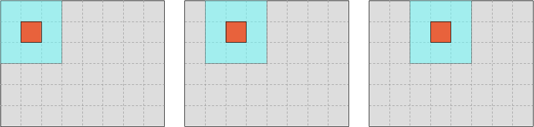
…where the gray rectangle represents the overall dataset, the blue square represents the location of the input values that we are reading at each step of the update loop, and the red square represents the location of the output value that we are writing at each step of the update loop.

Our goal in this chapter will be to instead iterate over wider (but equally high) input and output slices, where the output region is as wide as a hardware SIMD vector, and the input region follows by adding one data point on each side.

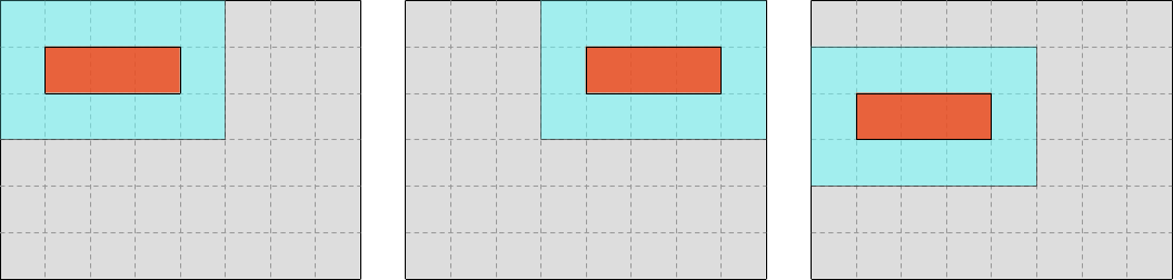
Once we get there, introducing SIMD will “just” be a matter of replacing each scalar operation in our algorithm with a SIMD operation that targets a SIMD vector starting at the same memory location.

Breaking the symmetry

This move to wider input and output windows is not without consequences, however. It breaks the symmetry between rows and columns that has existed so far in our computation, allowing us to perform 2D iteration over the dataset with a single, 1D-feeling loop.

Now we are going to need an outer loop over lines of output…

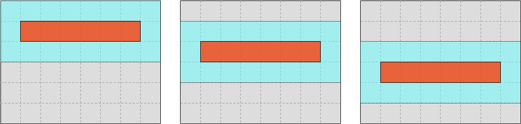
…and, under that outer loop, an inner loop over SIMD vectors within each line.

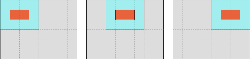
We are also going to need to decide how to handle the case where the number of output elements within a line is not a multiple of the SIMD vector length:

1. Do we simply forbid this to keep our code simple, at the cost of making users angry?
2. Do we handle the remaining elements of each line using a scalar computation?
3. Do we start by slicing up a “regular” part of the computation that has all the right properties for SIMD, processing the rest (including the edges of the simulation domain) using a more general but slower implementation?

There is no single right answer here, and the right way to go about this will depend on the technical and political specifics of the software that you are writing. But option 3 is a good tradeoff if you are unsure, and may therefore be a good starting point.

The “easy” part

We will now start implementing a subset of the update loop that only works on the part of the simulation domain that is easy to handle using SIMD.

First of all, assuming a pre-existing SIMD_WIDTH constant which contains our SIMD vector width, we can select an output region that covers all previous output rows, but only a number of columns that corresponds to an integer number of SIMD vectors:

use ndarray::s;

let [num_rows, num_cols] = start.shape();
let num_regular_cols = ((num_cols - 2) / SIMD_WIDTH) * SIMD_WIDTH;

let regular_output = s![1..(num_rows - 1), 1..=num_regular_cols];
let mut regular_out_u = end.u.slice_mut(regular_output);
let mut regular_out_v = end.v.slice_mut(regular_output);

let regular_input = s![0..num_rows, 0..=(num_regular_cols + 1)];
let regular_in_u = start.u.slice(regular_input);
let regular_in_v = start.v.slice(regular_input);

We can then iterate over rows of the output arrays and the corresponding windows of three consecutive input rows in the input arrays…

use ndarray::Axis;

let out_rows = (regular_out_u.rows_mut().into_iter()).zip(regular_out_v.rows_mut());

let in_windows = (regular_in_u.axis_windows(Axis(0), 3).into_iter())
    .zip(regular_in_v.axis_windows(Axis(0), 3));

// Cannot use `ndarray::azip` here because it does not support jointly
// iterating over ArrayViews of different dimensionality (here 1D and 2D)
for ((mut out_row_u, mut out_row_v), (win_u, win_v)) in out_rows.zip(in_windows) {
    // TODO: Process a row of output here
}

…and within that outer loop, we can have an inner loop on SIMD-sized chunks within each row of the output matrix, along with the corresponding input windows.

let out_chunks = (out_row_u.exact_chunks_mut(SIMD_WIDTH).into_iter())
    .zip(out_row_v.exact_chunks_mut(SIMD_WIDTH));

let in_windows = (win_u
    .axis_windows(Axis(1), SIMD_WIDTH + 2)
    .into_iter()
    .step_by(SIMD_WIDTH))
.zip(
    win_v
        .axis_windows(Axis(1), SIMD_WIDTH + 2)
        .into_iter()
        .step_by(SIMD_WIDTH),
);

// Cannot use `ndarray::azip` here for the same reason as before
for ((mut out_chunk_u, mut out_chunk_v), (win_u, win_v)) in out_chunks.zip(in_windows) {
    // TODO: Process a SIMD-sized chunk of output here
}

Finally, within the body of that inner loop, we can introduce a SIMD version of our regularized update algorithm, using std::simd:

use crate::data::Float;
use std::simd::prelude::*;

// Access the SIMD data corresponding to the center concentration
let simd_input = s![
    STENCIL_OFFSET[0],
    STENCIL_OFFSET[1]..SIMD_WIDTH + STENCIL_OFFSET[1],
];
let u = win_u.slice(simd_input);
let v = win_v.slice(simd_input);

// Load it as a SIMD vector
//
// The conversion from ArrayView to slice can fail if the data is
// not contiguous in memory. In this case, we know it should always
// be contiguous, so we can use unwrap() which panics otherwise.
type Vector = Simd<Float, SIMD_WIDTH>;
let u = Vector::from_slice(u.as_slice().unwrap());
let v = Vector::from_slice(v.as_slice().unwrap());

// Compute the diffusion gradient for U and V
let [full_u, full_v] = (win_u.windows([1, SIMD_WIDTH]).into_iter())
    .zip(win_v.windows([1, SIMD_WIDTH]))
    .zip(STENCIL_WEIGHTS.into_iter().flatten())
    .fold(
        [Vector::splat(0.); 2],
        |[acc_u, acc_v], ((stencil_u, stencil_v), weight)| {
            let stencil_u = Vector::from_slice(stencil_u.as_slice().unwrap());
            let stencil_v = Vector::from_slice(stencil_v.as_slice().unwrap());
            let weight = Vector::splat(weight);
            [
                acc_u + weight * (stencil_u - u),
                acc_v + weight * (stencil_v - v),
            ]
        },
    );

// Compute SIMD versions of all the float constants that we use
let diffusion_rate_u = Vector::splat(DIFFUSION_RATE_U);
let diffusion_rate_v = Vector::splat(DIFFUSION_RATE_V);
let feedrate = Vector::splat(opts.feedrate);
let killrate = Vector::splat(opts.killrate);
let deltat = Vector::splat(opts.deltat);
let ones = Vector::splat(1.0);

// Compute the output values of u and v
let uv_square = u * v * v;
let du = diffusion_rate_u * full_u - uv_square + feedrate * (ones - u);
let dv = diffusion_rate_v * full_v + uv_square - (feedrate + killrate) * v;
let out_u = u + du * deltat;
let out_v = v + dv * deltat;

// Store the output values of u and v
out_u.copy_to_slice(out_chunk_u.as_slice_mut().unwrap());
out_v.copy_to_slice(out_chunk_v.as_slice_mut().unwrap());

The main highlights here are that

• We can convert back from an ArrayView that has contiguous storage to a standard Rust slice for the purpose of interacting with the SIMD API, which doesn’t know about ndarray.
• We can still use 1D-like iteration in our inner diffusion gradient loop, it is only the outer loops on output elements that are affected by the change of algorithm.
• Floating point constants can be turned into SIMD vectors whose elements are all equal to the constant by using Simd::splat, which on x86 maps to the hardware broadcastss instruction.
• Adding SIMD to any nontrivial codebase without turning it into an unreadable mess is a major software engineering challenge¹.

Finally, because we are using the experimental nightly-only std::simd API, we will need to enable it by adding the associated #![feature(portable_simd)] directive to the top of exercises/src/lib.rs (assuming this is where you have put the update function’s implementation).

Exercise

Make a backup of your current update function, you will need some of it to handle the irregular subset of the data (simulation domain edges, extra columns that do not fit a SIMD vector nicely, etc).

Then integrate the above regularized SIMD algorithm into your code, and complete it by adding function multiversioning through the multiversion crate (as presented in the SIMD chapter), so that you get something to put inside of this SIMD_WIDTH constant:

const SIMD_WIDTH: usize = ...;

Finally, make your update function handle the irregular part of the simulation domain by reusing your former implementation.

Advanced SIMD

The SIMD version of the Gray-Scott simulation that we have implemented in the previous chapter has two significant issues that would be worth improving upon:

• The SIMD update loop is significantly more complex than the regularized scalar version.
• Its memory accesses suffer from alignment issues that will reduce runtime performance. On x86 specifically, at least 1 in 4 memory access¹ will be slowed down in SSE builds, 1 in 2 in AVX builds, and every memory access is in AVX-512 builds. So the more advanced your CPU’s SIMD instruction set, the worse the relative penalty becomes.

Interestingly, there is a way to improve the code on both of these dimensions, and simplify the update loop immensely while improving its runtime performance. However, there is no free lunch in programming, and we will need to pay a significant price in exchange for these improvements:

• The layout of numerical data in RAM will become less obvious and harder to reason about.
• Interoperability with other code that expects a more standard memory layout, such as the HDF5 I/O library, will become more difficult and have higher runtime overhead.
• We will need to give up on the idea that we can allow users to pick a simulation domain of any size they like, and enforce some hardware-originated constraints on the problem size.

Assuming these are constraints that you can live with, let us now get started!

A new data layout

So far, we have been laying out our 2D concentration data in the following straightforward manner:

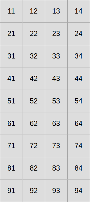
Now let us assume that we want to use SIMD vectors of width 3. We will start by slicing our scalar data into three equally tall horizontal slices, one per SIMD vector lane…

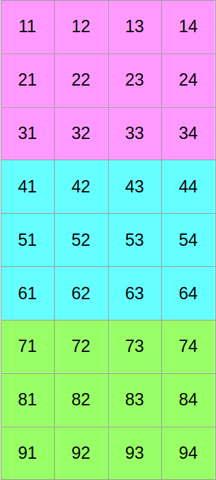
…and then we will shuffle around the data such that if we read it from left to right, we now get the first column of the former top block, followed by the first column of the middle block, followed by the first column of the bottom block, followed by the second column of the top block, and so on:

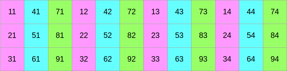
At this point, you may reasonably be skeptical that this is an improvement. But before you start doubting my sanity, let us look at the same data layout again, with a different visualization that emphasizes aligned SIMD vectors:

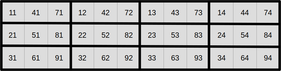
And now, let us assume that we want to compute the output aligned SIMD vector at coordinate (1, 1) from the top-left corner in this SIMD super-structure:

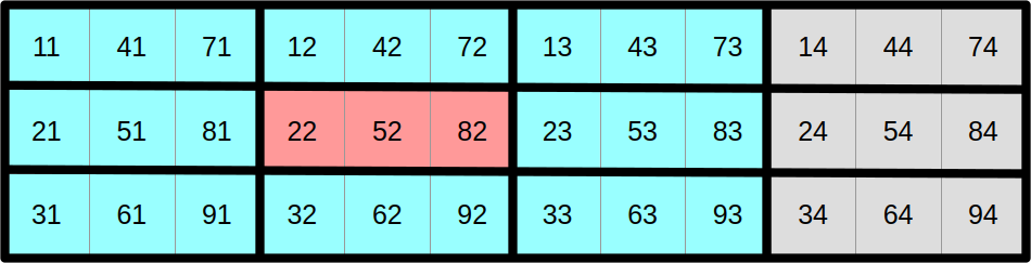
As it turns out, we can do it using a read and write pattern that looks exactly like the regularized scalar stencil that we have used before, but this time using correctly aligned SIMD vectors instead of scalar data points. Hopefully, by now, you will agree that we are getting somewhere.

Now that we have a very efficient data access pattern at the center of the simulation domain, let us reduce the need for special edge handling in order to make our simulation update loop even simpler. The left and right edges are easy, as we can just add zeroed out vectors on both sides and be careful not to overwrite them later in the computation…

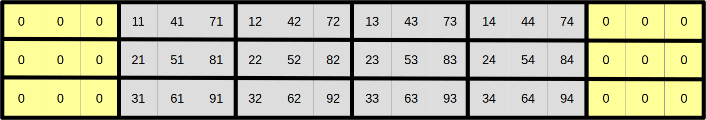
…but the top and bottom edges need more care. The upper neighbours of scalar elements at coordinates 1x is 0 and the lower neighbours of scalar elements at coordinates 9x are easy because they can also be permanently set to zero:

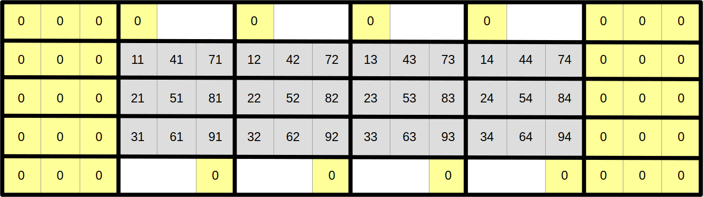
However, other top and bottom scalar elements will somehow need to wrap around the 2D array and shift by one column in order to access their upper and lower neighbors:

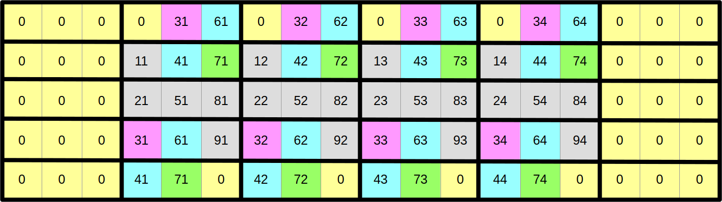
There are several ways to implement this wrapping around and column-shifting in a SIMD computation. In this course, we will use the approach of updating the upper and lower rows of the array after each computation step in order to keep them in sync with the matching rows at the opposite end of the array. This wrapping around and shifting will be done using an advanced family of SIMD instructions known as swizzles.

Even though SIMD swizzles are relatively expensive CPU instructions, especially on x86, their overhead will be imperceptible for sufficiently tall simulation domains. That’s because we will only need to use them in order to update the top and bottom rows of the simulation, no matter how many rows the simulation domain has, whereas the rest of the simulation update loop has a computational cost that grows linearly with the number of simulation domain rows.

Adjusting the code

Data layout changes can be an extremely powerful tool to optimize your code. And generally speaking there will always be a limit to how much performance you can gain without changing how data is laid out in files and in RAM.

But the motto of this course is that there is no free lunch in programming, and in this particular case, the price to pay for this change will be a major code rewrite to adapt almost every piece of code that we have previously written to the new data layout.²

U and V concentration storage

Our core UV struct has so far stored scalar data, but now we will make it store SIMD vectors instead. We want to do it for two reasons:

• It will make our SIMD update loop code much simpler and clearer.
• It will tell the compiler that we want to do SIMD with a certain width and the associated memory allocation should be correctly aligned for this purpose.

The data structure definition therefore changes to this:

use std::simd::{prelude::*, LaneCount, SupportedLaneCount};

/// Type alias for a SIMD vector of floats, we're going to use this type a lot
pub type Vector<const SIMD_WIDTH: usize> = Simd<Float, SIMD_WIDTH>;

/// Storage for the concentrations of the U and V chemical species
pub struct UV<const SIMD_WIDTH: usize>
where
    LaneCount<SIMD_WIDTH>: SupportedLaneCount,
{
    pub u: Array2<Vector<SIMD_WIDTH>>,
    pub v: Array2<Vector<SIMD_WIDTH>>,
}

Notice that the UV struct definition must now be generic over the SIMD vector width (reflecting the associated change in memory alignement in the underlying Array2s), and that this genericity must be bounded by a where clause³ to indicate that not all usizes are valid SIMD vector widths.⁴

The methods of the UV type change as well, since now the associated impl block must be made generic as well, and the implementation of the various methods must adapt to the fact that now our inner storage is made of SIMD vectors.

First the impl block will gain generics parameters, with bounds that match those of the source type:

impl<const SIMD_WIDTH: usize> UV<SIMD_WIDTH>
where
    LaneCount<SIMD_WIDTH>: SupportedLaneCount,
{
    // TODO: Add methods here
}

The reason why the impl blocks needs generics bounds as well is that this gives the language syntax headroom to let you add methods that are specific to one specific value of the generics parameters, like this:

impl UV<4> {
    // TODO: Add code specific to vectors of width 4 here
}

That being said, repeating bounds like this is certainly annoying in the common case, and there is a longstanding desire to add a way to tell the language “please just repeat the bounds of the type definitions”, using syntax like this:

impl UV<_> {
    // TODO: Add generic code that works for all SIMD_WIDTHS here
}

The interested reader is advised to use “implied bounds” as a search engine keyword, in order to learn more about how this could work, and why integrating this feature into Rust has not been as easy as initially envisioned.

The main UV::new() constructor changes a fair bit because it needs to account for the fact that…

1. There is now one extra SIMD vector on each side of the simulation domain
2. The SIMD-optimized data layout is quite different, and mapping our original rectangular concentration pattern to is is non-trivial.
3. To simplify this version of the code, we set the constraint that both the height and the width of the simulation domain must be a multiple of the SIMD vector width.

…which, when taken together, leads to this implementation:

fn new(num_scalar_rows: usize, num_scalar_cols: usize) -> Self {
    // Enforce constraints of the new data layout
    assert!(
        (num_scalar_rows % SIMD_WIDTH == 0) && (num_scalar_cols % SIMD_WIDTH == 0),
        "num_scalar_rows and num_scalar_cols must be a multiple of the SIMD vector width"
    );
    let num_center_rows = num_scalar_rows / SIMD_WIDTH;
    let simd_shape = [num_center_rows + 2, num_scalar_cols + 2];

    // Predicate which selects central rows and columns
    let is_center = |simd_row, simd_col| {
        simd_row >= 1
            && simd_row <= num_center_rows
            && simd_col >= 1
            && simd_col <= num_scalar_cols
    };

    // SIMDfied version of the scalar pattern, based on mapping SIMD vector
    // position and SIMD lane indices to equivalent positions in the
    // original scalar array.
    //
    // Initially, we zero out all edge elements. We will fix the top/bottom
    // elements in a later step.
    let pattern = |simd_row, simd_col| {
        let elements: [Float; SIMD_WIDTH] = if is_center(simd_row, simd_col) {
            std::array::from_fn(|simd_lane| {
                let scalar_row = simd_row - 1 + simd_lane * num_center_rows;
                let scalar_col = simd_col - 1;
                (scalar_row >= (7 * num_scalar_rows / 16).saturating_sub(4)
                    && scalar_row < (8 * num_scalar_rows / 16).saturating_sub(4)
                    && scalar_col >= 7 * num_scalar_cols / 16
                    && scalar_col < 8 * num_scalar_cols / 16) as u8 as Float
            })
        } else {
            [0.0; SIMD_WIDTH]
        };
        Vector::from(elements)
    };

    // The next steps are very similar to the scalar version...
    let u = Array2::from_shape_fn(simd_shape, |(simd_row, simd_col)| {
        if is_center(simd_row, simd_col) {
            Vector::splat(1.0) - pattern(simd_row, simd_col)
        } else {
            Vector::splat(0.0)
        }
    });
    let v = Array2::from_shape_fn(simd_shape, |(simd_row, simd_col)| {
        pattern(simd_row, simd_col)
    });
    let mut result = Self { u, v };

    // ...except we must fix up the top and bottom rows of the simulation
    // domain in order to achieve the intended data layout.
    result.update_top_bottom();
    result
}

Notice the call to the new update_top_bottom() method, which is in charge of calculating the top and bottom rows of the concentration array. We will get back to how this method works in a bit.

The all-zeroes constructor changes very little in comparison, since when everything is zero, the order of scalar elements within the array does not matter:

/// Set up an all-zeroes chemical species concentration
fn zeroes(num_scalar_rows: usize, num_scalar_cols: usize) -> Self {
    // Same idea as above
    assert!(
        (num_scalar_rows % SIMD_WIDTH == 0) && (num_scalar_cols % SIMD_WIDTH == 0),
        "num_scalar_rows and num_scalar_cols must be a multiple of the SIMD vector width"
    );
    let num_simd_rows = num_scalar_rows / SIMD_WIDTH;
    let simd_shape = [num_simd_rows + 2, num_scalar_cols + 2];
    let u = Array2::default(simd_shape);
    let v = Array2::default(simd_shape);
    Self { u, v }
}

The notion of shape becomes ambiguous in the new layout, because we need to clarify whether we are talking about the logical size of the simulation domain in scalar concentration data points, or its physical size in SIMD vector elements. Therefore, the former shape() method is split into two methods, and callers must be adapted to call the right method for their needs:

/// Get the number of rows and columns of the SIMD simulation domain
pub fn simd_shape(&self) -> [usize; 2] {
    let shape = self.u.shape();
    [shape[0], shape[1]]
}

/// Get the number of rows and columns of the scalar simulation domain
pub fn scalar_shape(&self) -> [usize; 2] {
    let [simd_rows, simd_cols] = self.simd_shape();
    [(simd_rows - 2) * SIMD_WIDTH, simd_cols - 2]
}

…and finally, we get to discuss the process through which the top and bottom rows of the SIMD concentration array are updated:

use multiversion::multiversion;
use ndarray::s;

// ...

/// Update the top and bottom rows of all inner arrays of concentrations
///
/// This method must be called between the end of a simulation update step
/// and the beginning of the next step to sync up the top/bottom rows of the
/// SIMD data store. It can also be used to simplify initialization.
fn update_top_bottom(&mut self) {
    // Due to a combination of language and compiler limitations, we
    // currently need both function multiversioning and genericity over SIMD
    // width here. See handouts for the full explanation.
    #[multiversion(targets("x86_64+avx2+fma", "x86_64+avx", "x86_64+sse2"))]
    fn update_array<const WIDTH: usize>(arr: &mut Array2<Vector<WIDTH>>)
    where
        LaneCount<WIDTH>: SupportedLaneCount,
    {
        // TODO: Implementation for one concentration array goes here
    }
    update_array(&mut self.u);
    update_array(&mut self.v);
}

First of all, we get this little eyesore of an inner function declaration:

#[multiversion(targets("x86_64+avx2+fma", "x86_64+avx", "x86_64+sse2"))]
fn update_array<const WIDTH: usize>(arr: &mut Array2<Vector<WIDTH>>)
where
    LaneCount<WIDTH>: SupportedLaneCount,
{
    // TODO: Top/bottom row update goes here
}

It needs to have a multiversion attribute AND a generic signature due to a combination of language and compiler limitations:

• Rust currently does not allow inner function declarations to access the generic parameters of outer functions. Therefore, the inner function must be made generic over WIDTH even though it will only be called for one specific SIMD_WIDTH.
• Genericity over SIMD_WIDTH is not enough to achieve optimal SIMD code generation, because by default, the compiler will only generate code for the lowest-common-denominator SIMD instruction set (SSE2 on x86_64), emulating wider vector widths using narrower SIMD operations. We still need function multi-versioning in order to generate one optimized code path per supported SIMD instruction set, and dispatch to the right code path at runtime.

Beyond that, the implementation is quite straightforward. First we extract the two top and bottom rows of the concentration array using ndarray slicing, ignoring the leftmost and rightmost element that we know to be zero…

// Select the top and bottom rows of the simulation domain
let shape = arr.shape();
let [num_simd_rows, num_cols] = [shape[0], shape[1]];
let horizontal_range = 1..(num_cols - 1);
let row_top = s![0, horizontal_range.clone()];
let row_after_top = s![1, horizontal_range.clone()];
let row_before_bottom = s![num_simd_rows - 2, horizontal_range.clone()];
let row_bottom = s![num_simd_rows - 1, horizontal_range];

// Extract the corresponding data slices
let (row_top, row_after_top, row_before_bottom, row_bottom) =
    arr.multi_slice_mut((row_top, row_after_top, row_before_bottom, row_bottom));

…and then we iterate over all SIMD vectors within the rows, generating “lane-shifted” versions using a combination of SIMD rotates and zero-assignment (which have wider hardware support than lane-shifting), and storing them on the opposite end of the array:

// Jointly iterate over all rows
ndarray::azip!((
    vec_top in row_top,
    &mut vec_after_top in row_after_top,
    &mut vec_before_bottom in row_before_bottom,
    vec_bottom in row_bottom
) {
    // Top vector acquires the value of the before-bottom vector,
    // rotated right by one lane and with the first element set to zero
    let mut shifted_before_bottom = vec_before_bottom.rotate_elements_right::<1>();
    shifted_before_bottom[0] = 0.0;
    *vec_top = shifted_before_bottom;

    // Bottom vector acquires the value of the after-top vector, rotated
    // left by one lane and with the last element set to zero
    let mut shifted_after_top = vec_after_top.rotate_elements_left::<1>();
    shifted_after_top[WIDTH - 1] = 0.0;
    *vec_bottom = shifted_after_top;
});

Double buffering and the SIMD-scalar boundary

Because our new concentration storage has become generic over the width of the SIMD instruction set in use, our double buffer abstraction must become generic as well:

pub struct Concentrations<const SIMD_WIDTH: usize>
where
    LaneCount<SIMD_WIDTH>: SupportedLaneCount,
{
    buffers: [UV<SIMD_WIDTH>; 2],
    src_is_1: bool,
}

However, now is a good time to ask ourselves where we should put the boundary of code which must know about this genericity and the associated SIMD data storage. We do not want to simply propagate SIMD types everywhere because…

1. It would make all the code generic, which as we have seen is a little annoying, and also slows compilation down (all SIMD-generic code is compiled once per possible hardware vector width).
2. Some of our dependencies like hdf5 are lucky enough not to know or care about SIMD data types. At some point, before we hand over data to these dependencies, a conversion to the standard scalar layout will need to be performed.

Right now, the only point where the Concentrations::current() method is used is when we hand over the current value of V species concentration array to HDF5 for the purpose of writing it out. Therefore, it is reasonable to use this method as our SIMD-scalar boundary by turning it into a current_v() method that returns a scalar view of the V concentration array, which is computed on the fly whenever requested.

We can prepare for this by adding a new scalar array member to the Concentrations struct…

pub struct Concentrations<const SIMD_WIDTH: usize>
where
    LaneCount<SIMD_WIDTH>: SupportedLaneCount,
{
    buffers: [UV<SIMD_WIDTH>; 2],
    src_is_1: bool,
    scalar_v: Array2<Float>,  // <- New
}

…and zero-initializing it in the Concentrations::new() constructor:

/// Set up the simulation state
pub fn new(num_scalar_rows: usize, num_scalar_cols: usize) -> Self {
    Self {
        buffers: [
            UV::new(num_scalar_rows, num_scalar_cols),
            UV::zeroes(num_scalar_rows, num_scalar_cols),
        ],
        src_is_1: false,
        scalar_v: Array2::zeros([num_scalar_rows, num_scalar_cols]),  // <- New
    }
}

And finally, we must turn current() into current_v(), make it take &mut self instead of &self so that it can mutate the internal buffer, and make it return a reference to the internal buffer:

/// Read out the current V species concentration
pub fn current_v(&mut self) -> &Array2<Float> {
    let simd_v = &self.buffers[self.src_is_1 as usize].v;
    // TODO: Compute scalar_v from simd_v
    &self.scalar_v
}

The rest of the double buffer does not change much, it is just a matter of…

• Adding generics in the right place
• Exposing new API distinctions that didn’t exist before between the scalar domain shape and the SIMD domain shape
• Updating the top and bottom rows of the SIMD dataset after each update.

impl<const SIMD_WIDTH: usize> Concentrations<SIMD_WIDTH>
where
    LaneCount<SIMD_WIDTH>: SupportedLaneCount,
{
    /// Set up the simulation state
    pub fn new(num_scalar_rows: usize, num_scalar_cols: usize) -> Self {
        Self {
            buffers: [
                UV::new(num_scalar_rows, num_scalar_cols),
                UV::zeroes(num_scalar_rows, num_scalar_cols),
            ],
            src_is_1: false,
            scalar_v: Array2::zeros([num_scalar_rows, num_scalar_cols]),
        }
    }

    /// Get the number of rows and columns of the SIMD simulation domain
    pub fn simd_shape(&self) -> [usize; 2] {
        self.buffers[0].simd_shape()
    }

    /// Get the number of rows and columns of the scalar simulation domain
    pub fn scalar_shape(&self) -> [usize; 2] {
        self.buffers[0].scalar_shape()
    }

    /// Read out the current V species concentration
    pub fn current_v(&mut self) -> &Array2<Float> {
        let simd_v = &self.buffers[self.src_is_1 as usize].v;
        // TODO: Compute scalar_v from simd_v
        &self.scalar_v
    }

    /// Run a simulation step
    ///
    /// The user callback function `step` will be called with two inputs UVs:
    /// one containing the initial species concentration at the start of the
    /// simulation step, and one to receive the final species concentration that
    /// the simulation step is in charge of generating.
    ///
    /// The `step` callback needs not update the top and the bottom rows of the
    /// SIMD arrays, it will be updated automatically.
    pub fn update(&mut self, step: impl FnOnce(&UV<SIMD_WIDTH>, &mut UV<SIMD_WIDTH>)) {
        let [ref mut uv_0, ref mut uv_1] = &mut self.buffers;
        if self.src_is_1 {
            step(uv_1, uv_0);
            uv_0.update_top_bottom();
        } else {
            step(uv_0, uv_1);
            uv_1.update_top_bottom();
        }
        self.src_is_1 = !self.src_is_1;
    }
}

But of course, there is a big devil in that TODO detail within the implementation of current_v().

Going back to the scalar data layout

Let us go back to the virtual drawing board and fetch back our former schematic that illustrates the mapping between the SIMD and scalar data layout:

It may not be clear from a look at it, but given a set of SIMD_WIDTH consecutive vectors of SIMD data, it is possible to efficiently reconstruct a SIMD_WIDTH vectors of scalar data.

In other words, there are reasonably efficient SIMD instructions for performing this transformation:

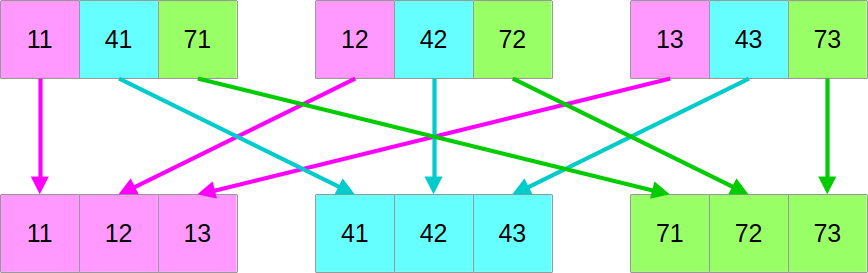
Unfortunately, the logic of these instructions is highly hardware-dependent, and Rust’s std::simd has so far shied away from implementing higher-level abstract operations that involve more than two input SIMD vectors. Therefore, we will have to rely on autovectorization for this as of today.

Also, to avoid complicating the code with a scalar fallback, we should enforce that the number of columns in the underlying scalar array is a multiple of SIMD_WIDTH. Which is reasonable given that we already enforce this for the number of rows. This is already done in the UV constructors that you have been provided with above.

But given these two prerequisites, here is a current_v() implementation that does the job:

use ndarray::ArrayView2;

// ...

/// Read out the current V species concentration
pub fn current_v(&mut self) -> &Array2<Float> {
    // Extract the center region of the V input concentration table
    let uv = &self.buffers[self.src_is_1 as usize];
    let [simd_rows, simd_cols] = uv.simd_shape();
    let simd_v_center = uv.v.slice(s![1..simd_rows - 1, 1..simd_cols - 1]);

    // multiversion does not support methods that take `self` yet, so we must
    // use an inner function for now.
    #[multiversion(targets("x86_64+avx2+fma", "x86_64+avx", "x86_64+sse2"))]
    fn make_scalar<const WIDTH: usize>(
        simd_center: ArrayView2<Vector<WIDTH>>,
        scalar_output: &mut Array2<Float>,
    ) where
        LaneCount<WIDTH>: SupportedLaneCount,
    {
        // Iterate over SIMD rows...
        let simd_center_rows = simd_center.nrows();
        for (simd_row_idx, row) in simd_center.rows().into_iter().enumerate() {
            // ...and over chunks of WIDTH vectors within each rows
            for (simd_chunk_idx, chunk) in row.exact_chunks(WIDTH).into_iter().enumerate() {
                // Convert this chunk of SIMD vectors to the scalar layout,
                // relying on autovectorization for performance for now...
                let transposed: [[Float; WIDTH]; WIDTH] = std::array::from_fn(|outer_idx| {
                    std::array::from_fn(|inner_idx| chunk[inner_idx][outer_idx])
                });

                // ...then store these scalar vectors in the right location
                for (vec_idx, data) in transposed.into_iter().enumerate() {
                    let scalar_row = simd_row_idx + vec_idx * simd_center_rows;
                    let scalar_col = simd_chunk_idx * WIDTH;
                    scalar_output
                        .slice_mut(s![scalar_row, scalar_col..scalar_col + WIDTH])
                        .as_slice_mut()
                        .unwrap()
                        .copy_from_slice(&data)
                }
            }
        }
    }
    make_scalar(simd_v_center.view(), &mut self.scalar_v);

    // Now scalar_v contains the scalar version of v
    &self.scalar_v
}

As you may guess, this implementation could be optimized further…

• The autovectorized transpose could be replaced with hardware-specific SIMD swizzles.
• The repeated slicing of scalar_v could be replaced with a set of iterators that yield the right output chunks without any risk of unelided bounds checks.

…but given that even the most optimized data transpose is going to be costly due to how hardware works, it would probably best to optimize by simply saving scalar output less often!

The new simulation kernel

Finally, after going through all of this trouble, we can adapt the heart of the simulation, the update() loop, to the new data layout:

use std::simd::{LaneCount, SupportedLaneCount};

/// Simulation update function
#[multiversion(targets("x86_64+avx2+fma", "x86_64+avx", "x86_64+sse2"))]
pub fn update<const SIMD_WIDTH: usize>(
    opts: &UpdateOptions,
    start: &UV<SIMD_WIDTH>,
    end: &mut UV<SIMD_WIDTH>,
) where
    LaneCount<SIMD_WIDTH>: SupportedLaneCount,
{
    let [num_simd_rows, num_simd_cols] = start.simd_shape();
    let output_range = s![1..=(num_simd_rows - 2), 1..=(num_simd_cols - 2)];
    ndarray::azip!((
        win_u in start.u.windows([3, 3]),
        win_v in start.v.windows([3, 3]),
        out_u in end.u.slice_mut(output_range),
        out_v in end.v.slice_mut(output_range),
    ) {
        // Access the SIMD data corresponding to the center concentration
        let u = win_u[STENCIL_OFFSET];
        let v = win_v[STENCIL_OFFSET];

        // Compute the diffusion gradient for U and V
        let [full_u, full_v] = (win_u.into_iter())
            .zip(win_v)
            .zip(STENCIL_WEIGHTS.into_iter().flatten())
            .fold(
                [Vector::splat(0.); 2],
                |[acc_u, acc_v], ((stencil_u, stencil_v), weight)| {
                    let weight = Vector::splat(weight);
                    [
                        acc_u + weight * (stencil_u - u),
                        acc_v + weight * (stencil_v - v),
                    ]
                },
            );

        // Compute SIMD versions of all the float constants that we use
        let diffusion_rate_u = Vector::splat(DIFFUSION_RATE_U);
        let diffusion_rate_v = Vector::splat(DIFFUSION_RATE_V);
        let feedrate = Vector::splat(opts.feedrate);
        let killrate = Vector::splat(opts.killrate);
        let deltat = Vector::splat(opts.deltat);
        let ones = Vector::splat(1.0);

        // Compute the output values of u and v
        let uv_square = u * v * v;
        let du = diffusion_rate_u * full_u - uv_square + feedrate * (ones - u);
        let dv = diffusion_rate_v * full_v + uv_square - (feedrate + killrate) * v;
        *out_u = u + du * deltat;
        *out_v = v + dv * deltat;
    });
}

Notice the following:

• This code looks a lot simpler and closer to the regularized scalar code than the previous SIMD code which tried to adjust to the scalar data layout. And that’s all there is to it. No need for a separate update code path to handle the edges of the simulation domain!
• The SIMD vector width is not anymore an implementation detail that can be contained within the scope of this function, as it appears in the input and output types. Therefore, function multiversioning alone is not enough and we need genericity over the SIMD width too.

Adapting run_simulation() and the HDF5Writer

The remaining changes in the shared computation code are minor. Since our simulation runner allocates the concentration arrays, it must now become generic over the SIMD vector type and adapt to the new Concentrations API…

/// Simulation runner, with a user-specified concentration update function
pub fn run_simulation<const SIMD_WIDTH: usize>(
    opts: &RunnerOptions,
    // Notice that we must use FnMut here because the update function can be
    // called multiple times, which FnOnce does not allow.
    mut update: impl FnMut(&UV<SIMD_WIDTH>, &mut UV<SIMD_WIDTH>),
) -> hdf5::Result<()>
where
    LaneCount<SIMD_WIDTH>: SupportedLaneCount,
{
    // Set up the concentrations buffer
    let mut concentrations = Concentrations::new(opts.num_rows, opts.num_cols);

    // Set up HDF5 I/O
    let mut hdf5 = HDF5Writer::create(
        &opts.file_name,
        concentrations.scalar_shape(),
        opts.num_output_steps,
    )?;

    // Produce the requested amount of concentration arrays
    for _ in 0..opts.num_output_steps {
        // Run a number of simulation steps
        for _ in 0..opts.compute_steps_per_output_step {
            // Update the concentrations of the U and V chemical species
            concentrations.update(&mut update);
        }

        // Write down the current simulation output
        hdf5.write(concentrations.current_v())?;
    }

    // Close the HDF5 file
    hdf5.close()
}

…while the write() method of the HDF5Writer must adapt to the fact that it now only has access to the V species’ concentration, not the full dataset:

use ndarray::Array2;

// ...

/// Write a new V species concentration array to the file
pub fn write(&mut self, result_v: &Array2<Float>) -> hdf5::Result<()> {
    self.dataset
        .write_slice(result_v, (self.position, .., ..))?;
    self.position += 1;
    Ok(())
}

Exercise

Integrate all of these changes into your code repository. Then adjust both the microbenchmark at benches/simulate.rs and the main simulation binary at src/bin/simulate.rs to call the new run_simulation() and update() function.

You will need to use one final instance of function multiversioning in order to determine the appropriate SIMD_WIDTH inside of the top-level binaries. See our initial SIMD chapter for an example of how this is done.

In the case of microbenchmarks, you will also need to tune the loop on problem sizes in order to stop running benchmarks on the 4x4 problem size, which is not supported by this implementation.

Add a microbenchmark that measures the overhead of converting data from the SIMD to the scalar data layout, complementing the simulation update microbenchmark that you already have.

And finally, measure the impact of the new data layout on the performance of simulation updates.

Unfortunately, you may find the results to be a little disappointing. The why and how of this disappointment will be covered in the next chapter.

An inlining puzzle

A major promise of C++, which was inherited by Rust, is that it should be possible to write reasonably straightforward high-level code, which compiles down to highly optimized machine code, by virtue of providing the compiler optimizer with all the information it needs to remove the high-level abstraction overhead at compile time.

Unfortunately, this promise comes with a footnote concerning function inlining:

• The process of turning high-level abstractions into efficient machine code vitally depends on a particular compiler optimization known as inline expansion or inlining. This optimization revolves around strategically copying and pasting the code of a function into its callers when it seems worthwhile, which enables many more optimizations down the line by letting the compiler specialize the function’s code for the context in which it is being called.
• Compiler optimizers decide whether to inline a function or not based on heuristics, and sometimes the heuristics is wrong and decides not to inline a function which should be inlined. This can result in an enormous runtime performance penalty.

In our case, as a quick run through a profiler will tell you, the performance problems that were observed at the end of the last chapter come from the fact that the compiler did not inline some iterator-related functions that are key to our code’s performance.

Available tools for inlining issues

When the function that is not inlined is a function that you wrote, there is an easy fix. Just annotate the function that fails to inline properly with an #[inline]. This will adjust the compiler optimizer’s cost model concerning this function, and increase the odds that it does get inlined.

Most of the time, using #[inline] will be enough to restore inlining where it should happen, and bring back the runtime performance that you would expect. But unfortunately, #[inline] is just a hint, and the compiler’s optimizer may occasionally refuse to take the hint and insist that in its machine-opinion, a function really should not be inlined.

For those difficult situations, Rust provides you with #[inline(always)], which is a much stronger hint that a function should always be inlined, even in debug builds. Basically, if it is at all possible to inline a function that is annotated with #[inline(always)]¹, the compiler will inline it.

Unfortunately, while all of this is useful, it does not address one important use case: what should you do when the function that fails to inline is not in your code, but in a different library like one of your dependencies or the standard library, as happens in our case?

When this happens, you basically have three options:

1. Get in touch with the developers of that library and try to get them to add #[inline] directives in the right place. This works, but can take a while, and may fail if the authors of the library are not convinced that most users need inlining for runtime performance.²
2. Tweak the code in the hope of getting it into a shape that inlines better.
3. Roll your own version of the affected function(s), applying as much inlining directives as necessary to get the performance that you want.

For practical reasons³, this chapter will cover the last two options.

Locating the bad inlining

The inlining failures that are killing our performance stick out in the output of perf report.

There are two hot functions here that should be inlined into their caller, but are not:

• The next() method of our zipped iterator over window elements and stencil weights. Failing to inline this will increase the cost of each loop iteration by some amount, since now iteration variables will need to be pushed to the stack and popped back when they could stay resident in CPU registers instead. This is already quite bad in such a tight loop.
• The ndarray::zip::Zip::inner() method that performs the iteration over zipped iterators and does the actual computation is the biggest problem, however. Failing to inline this function into its multi-versioned caller breaks function multi-versioning, because the out-lined version will not be multiversioned. Therefore, it will only be compiled for the lowest denominator x86_64 SIMD instruction set of SSE2, which will cost us a lot of SIMD performance.

The first issue is actually surprisingly easy to resolve, once you know the trick. Just replace the 1D-style flattened iterator that makes the compiler optimizer choke with a version that separates the iteration over rows and columns of data:

// We give up on this...
(win_u.into_iter())
    .zip(win_v)
    .zip(STENCIL_WEIGHTS.into_iter().flatten())

// ...and instead go for this:
(win_u.rows().into_iter())
    .zip(win_v.rows())
    .zip(STENCIL_WEIGHTS)
    .flat_map(|((u_row, v_row), weights_row)| {
        (u_row.into_iter().copied())
            .zip(v_row.into_iter().copied())
            .zip(weights_row)
    })

As it turns out, the compiler has an easier time inlining through two layers of simple iteration than one layer of complex iteration, which is annoying but fair enough.

The second issue, however, is more difficult to resolve. ndarray’s producer-zipping code is quite complex because it tries to support arrays of arbitrary dimensionality, storage backend, and layout. Therefore, the amount of code that would need to be marked #[inline] would be quite large, and there is a relatively high risk that upstream would reject an associated pull request because it could have unforeseen side-effects on other code that calls ndarray::azip!().⁴

Hence we are going to go for a different approach, and instead roll our own 4-arrays-zipping iterator that is specialized for our needs… and marked #[inline] the way we want it.

Introducing unsafe

A key design goal of Rust is that most of the code that you write should be proven to be type-safe, memory-safe and thread-safe, either at compile time or via runtime checks. For concision reasons, code that achieves the combination of these three properties is referred to as “safe code”.

Sadly, Rust cannot extend this proof to 100% of your code for two important reasons:

• There are useful software operations whose correctness cannot be proven at compile-time. Think about, for example, calling into a third-party library that is implemented in C/++. Since code written in these languages is not proven to be safe at compile time and does not formally document its runtime safety invariants, there is no way for the Rust compiler to prove that such a function call is safe. Yet being able to interoperate with the existing ecosystem of C/++ code is a very important asset that most Rust programmers would not want to give up on.
• Runtime checks come at a runtime performance cost, unless they are eliminated by the compiler’s optimizer. Unfortunately, compiler optimizers are not very good at this job, and it is very common for them to leave around runtime safety checks in situations where a human could easily prove that they will never be triggered. The associated performance cost may not be acceptable to programs with strict runtime performance requirements.

As a compromise, Rust therefore provides access to supplementary operations of unproven safety, whose use is guarded by the unsafe keyword. They have various uses, but for our purposes, the operations of highest interest will be those that replicate standard library constructs that involve safety checks, but without the safety checks. Instead of crashing the program at runtime on erronerous usage, these unsafe operations will instead trigger undefined behavior and let the compiler trash your program in unpredictable ways, like most C/++ operations do.

The intended use of these unsafe operations is of course not to make Rust a C/++-like undefined behavior free-for-all, turning all of the hard-earned language safety guarantees into a fragile illusion that shatters on the first use of the unsafe keyword. Instead, unsafe operations are meant to be used inside by the implementation of safe operations³, in order to do things that the safe subset of the language cannot currently do due to compiler limitations, like safely indexing into arrays at a known-good position without paying the price of runtime bound checks.

As you may guess by now, the iterators of all basic collection types (arrays, Vecs…) are implemented using unsafe code. And so are the iterators of ndarray’s multidimensional arrays.

Of course, use of unsafe code is not without risks. The human proof backing the implementation of safe operations may be wrong, and let the risk of Undefined Behavior (UB) slip through, which is why frivolous use of unsafe is highly frowned upon in the Rust community. In a nutshell, unsafe code authors must keep in mind that…

• unsafe code should only be used in situations where there is no safe way to perform the task. The Rust community’s tolerance for convoluted safe code that improve compiler optimizations through unnatural contortions is much higher than for unsafe code that could be safe.
• If a function is not marked as unsafe, there must be no combination of inputs that can lead to the emergence of undefined behavior when it is called.
• If a function is marked as unsafe, its documentation must clearly spell out the safety contract that must be followed to avoid undefined behavior. This is needed so that users of the unsafe function know how to correctly use it later on.

An optimized iterator

This is an optimized version of our lockstep iteration pattern, implemented using unsafe code:

use ndarray::{ArrayView2, ShapeBuilder};

/// Optimized iterator over stencil output locations and input windows
#[inline]
pub fn stencil_iter<'data, const SIMD_WIDTH: usize>(
    start: &'data UV<SIMD_WIDTH>,
    end: &'data mut UV<SIMD_WIDTH>,
) -> impl Iterator<
    Item = (
        ArrayView2<'data, Vector<SIMD_WIDTH>>, // <- Input u window
        ArrayView2<'data, Vector<SIMD_WIDTH>>, // <- Input v window
        &'data mut Vector<SIMD_WIDTH>,         // <- Output u
        &'data mut Vector<SIMD_WIDTH>,         // <- Output v
    ),
>
where
    LaneCount<SIMD_WIDTH>: SupportedLaneCount,
{
    // Assert that the sub-grids all have the same memory layout.
    // This means that what we learn about one is valid for the other.
    //
    // It is fine to have a bunch of runtime assertions in an iterator
    // constructor, because their cost will be amortized across all iterations.
    assert_eq!(start.u.shape(), start.v.shape());
    assert_eq!(start.u.shape(), end.u.shape());
    assert_eq!(start.u.shape(), end.v.shape());
    assert_eq!(start.u.strides(), start.v.strides());
    assert_eq!(start.u.strides(), end.u.strides());
    assert_eq!(start.u.strides(), end.v.strides());

    // Collect and check common layout information
    let in_shape = start.simd_shape();
    assert!(in_shape.into_iter().min().unwrap() >= 2);
    let strides = start.u.strides();
    assert_eq!(strides.len(), 2);
    assert!(strides.iter().all(|stride| *stride > 0));
    let [row_stride, col_stride] = [strides[0] as usize, strides[1] as usize];
    assert_eq!(col_stride, 1);

    // Select the center of the simulation domain
    let out_shape = in_shape.map(|dim| dim - 2);
    let out_slice = s![1..=out_shape[0], 1..out_shape[1]];
    let mut out_u = end.u.slice_mut(out_slice);
    let mut out_v = end.v.slice_mut(out_slice);
    assert_eq!(start.u.strides(), out_u.strides());
    assert_eq!(start.u.strides(), out_v.strides());
    let [out_rows, out_cols] = out_shape;

    // Determine how many elements we must skip in order to go from the
    // past-the-end element of one row to the first element of the next row.
    let next_row_step = row_stride - out_cols;

    // Prepare a way to access input windows and output refs by output position
    // The safety of the closures below is actually asserted on the caller's
    // side, but sadly unsafe closures aren't a thing in Rust yet.
    let stencil_shape = [STENCIL_WEIGHTS.len(), STENCIL_WEIGHTS[0].len()];
    let window_shape = (stencil_shape[0], stencil_shape[1]).strides((row_stride, 1));
    let unchecked_output = move |out_ptr: *mut Vector<SIMD_WIDTH>| unsafe { &mut *out_ptr };
    let unchecked_input_window = move |in_ptr: *const Vector<SIMD_WIDTH>| unsafe {
        ArrayView2::from_shape_ptr(window_shape, in_ptr)
    };

    // Recipe to emit the currently selected input windows and output references,
    // then move to the next column. As before, this is only safe if called with
    // correct element pointers.
    let emit_and_increment =
        move |in_u_ptr: &mut *const Vector<SIMD_WIDTH>,
              in_v_ptr: &mut *const Vector<SIMD_WIDTH>,
              out_u_ptr: &mut *mut Vector<SIMD_WIDTH>,
              out_v_ptr: &mut *mut Vector<SIMD_WIDTH>| unsafe {
            let win_u = unchecked_input_window(*in_u_ptr);
            let win_v = unchecked_input_window(*in_v_ptr);
            let out_u = unchecked_output(*out_u_ptr);
            let out_v = unchecked_output(*out_v_ptr);
            *in_u_ptr = in_u_ptr.add(1);
            *in_v_ptr = in_v_ptr.add(1);
            *out_u_ptr = out_u_ptr.add(1);
            *out_v_ptr = out_v_ptr.add(1);
            (win_u, win_v, out_u, out_v)
        };

    // Set up iteration state
    let mut in_u_ptr = start.u.as_ptr();
    let mut in_v_ptr = start.v.as_ptr();
    let mut out_u_ptr = out_u.as_mut_ptr();
    let mut out_v_ptr = out_v.as_mut_ptr();
    //
    // End of the current row processed by out_v_ptr
    let mut out_v_row_end = unsafe { out_v_ptr.add(out_cols) };
    //
    // End of the last row of the output grid
    let out_v_end = unsafe { out_v_row_end.add(out_rows.saturating_sub(1) * row_stride) };

    // Emit output iterator
    std::iter::from_fn(move || {
        // Common case : we are within the bounds of a row and advance normally
        if out_v_ptr < out_v_row_end {
            return Some(emit_and_increment(
                &mut in_u_ptr,
                &mut in_v_ptr,
                &mut out_u_ptr,
                &mut out_v_ptr,
            ));
        }

        // Otherwise, check if we reached the end of iteration
        if out_v_ptr == out_v_end {
            return None;
        }

        // We're at the end of a row, but not at the end of iteration:
        // switch to the next row then emit the next element as usual
        debug_assert_eq!(out_v_ptr, out_v_row_end);
        unsafe {
            in_u_ptr = in_u_ptr.add(next_row_step);
            in_v_ptr = in_v_ptr.add(next_row_step);
            out_u_ptr = out_u_ptr.add(next_row_step);
            out_v_ptr = out_v_ptr.add(next_row_step);
            out_v_row_end = out_v_ptr.add(out_cols);
        }
        Some(emit_and_increment(
            &mut in_u_ptr,
            &mut in_v_ptr,
            &mut out_u_ptr,
            &mut out_v_ptr,
        ))
    })
}

We do not have the time to cover how it works in detail, but in a nutshell, it is the same code that the iterator zip in our optimized SIMD implementation should compile down to, and unlike the iterator zip, we wrote it and therefore can put a hard-earned #[inline] directive on it.

Exercise

Integrate these two iterator inlining optimizations into your code, and measure their effect on runtime performance. It should now be more in line (heh heh) with what you would expect considering the work that was put into SIMD layout improvements in the last chapter.

There is a lesson to be learned here: when an optimization does not have the payoff that you would expect, do not conclude that it is bad right away. Instead, take the time to figure out what’s going on, and whether your optimization is truly working as intended.

FMA vs ILP

If you paid close attention during the first part of this course, you may have been thinking for a while now that there is some code in the Gray-Scott computation that looks like a perfect candidate for introducing fused multiply-add CPU instructions.

More specifically, if we look at an iteration of the update loop…

// Access the SIMD data corresponding to the center concentration
let u = win_u[STENCIL_OFFSET];
let v = win_v[STENCIL_OFFSET];

// Compute the diffusion gradient for U and V
let [full_u, full_v] = (win_u.rows().into_iter())
    .zip(win_v.rows())
    .zip(STENCIL_WEIGHTS)
    .flat_map(|((u_row, v_row), weights_row)| {
        (u_row.into_iter().copied())
            .zip(v_row.into_iter().copied())
            .zip(weights_row)
    })
    .fold(
        [Vector::splat(0.); 2],
        |[acc_u, acc_v], ((stencil_u, stencil_v), weight)| {
            let weight = Vector::splat(weight);
            [
                acc_u + weight * (stencil_u - u),
                acc_v + weight * (stencil_v - v),
            ]
        },
    );

// Compute SIMD versions of all the float constants that we use
let diffusion_rate_u = Vector::splat(DIFFUSION_RATE_U);
let diffusion_rate_v = Vector::splat(DIFFUSION_RATE_V);
let feedrate = Vector::splat(opts.feedrate);
let killrate = Vector::splat(opts.killrate);
let deltat = Vector::splat(opts.deltat);
let ones = Vector::splat(1.0);

// Compute the output values of u and v
let uv_square = u * v * v;
let du = diffusion_rate_u * full_u - uv_square + feedrate * (ones - u);
let dv = diffusion_rate_v * full_v + uv_square - (feedrate + killrate) * v;
*out_u = u + du * deltat;
*out_v = v + dv * deltat;

…we can see that the diffusion gradient’s fold() statement and the computation of the output values of u and v are full of floating point multiplications followed by additions.

It would surely seem sensible to replace these with fused multiply-add operations that compute multiplication-addition pairs 2x faster and more accurately at the same time!

Free lunch at last?

Enticed by the prospect of getting an easy 2x performance speedup at last, we proceed to rewrite all the code using fused multiply-add operations…

// We must bring this trait in scope in order to use mul_add()
use std::simd::StdFloat;

// Compute the diffusion gradient for U and V
let [full_u, full_v] = (win_u.rows().into_iter())
    .zip(win_v.rows())
    .zip(STENCIL_WEIGHTS)
    .flat_map(|((u_row, v_row), weights_row)| {
        (u_row.into_iter().copied())
            .zip(v_row.into_iter().copied())
            .zip(weights_row)
    })
    .fold(
        [Vector::splat(0.); 2],
        |[acc_u, acc_v], ((stencil_u, stencil_v), weight)| {
            let weight = Vector::splat(weight);
            [
                // NEW: Introduced FMA here
                (stencil_u - u).mul_add(weight, acc_u),
                (stencil_v - v).mul_add(weight, acc_v),
            ]
        },
    );

// Compute SIMD versions of all the float constants that we use
let diffusion_rate_u = Vector::splat(DIFFUSION_RATE_U);
let diffusion_rate_v = Vector::splat(DIFFUSION_RATE_V);
let feedrate = Vector::splat(opts.feedrate);
let killrate = Vector::splat(opts.killrate);
let deltat = Vector::splat(opts.deltat);
let ones = Vector::splat(1.0);

// Compute the output values of u and v
// NEW: Introduced even more FMA there
let uv_square = u * v * v;
let du = diffusion_rate_u.mul_add(full_u, (ones - u).mul_add(feedrate, -uv_square));
let dv = diffusion_rate_v.mul_add(full_v, -(feedrate + killrate).mul_add(v, uv_square));
*out_u = du.mul_add(deltat, u);
*out_v = dv.mul_add(deltat, v);

…and we run our microbenchmarks, full of hope…

simulate/16x16          time:   [8.3555 µs 8.3567 µs 8.3580 µs]
                        thrpt:  [30.629 Melem/s 30.634 Melem/s 30.638 Melem/s]
                 change:
                        time:   [+731.23% +731.59% +731.89%] (p = 0.00 < 0.05)
                        thrpt:  [-87.979% -87.975% -87.970%]
                        Performance has regressed.
Found 9 outliers among 100 measurements (9.00%)
  6 (6.00%) high mild
  3 (3.00%) high severe
simulate/64x64          time:   [68.137 µs 68.167 µs 68.212 µs]
                        thrpt:  [60.048 Melem/s 60.088 Melem/s 60.114 Melem/s]
                 change:
                        time:   [+419.07% +419.96% +421.09%] (p = 0.00 < 0.05)
                        thrpt:  [-80.809% -80.768% -80.735%]
                        Performance has regressed.
Found 4 outliers among 100 measurements (4.00%)
  1 (1.00%) high mild
  3 (3.00%) high severe
Benchmarking simulate/256x256: Warming up for 3.0000 s
Warning: Unable to complete 100 samples in 5.0s. You may wish to increase target time to 8.7s, enable flat sampling, or reduce sample count to 50.
simulate/256x256        time:   [891.62 µs 891.76 µs 891.93 µs]
                        thrpt:  [73.476 Melem/s 73.491 Melem/s 73.502 Melem/s]
                 change:
                        time:   [+327.65% +329.35% +332.59%] (p = 0.00 < 0.05)
                        thrpt:  [-76.883% -76.709% -76.616%]
                        Performance has regressed.
Found 10 outliers among 100 measurements (10.00%)
  2 (2.00%) high mild
  8 (8.00%) high severe
simulate/1024x1024      time:   [10.769 ms 11.122 ms 11.489 ms]
                        thrpt:  [91.266 Melem/s 94.276 Melem/s 97.370 Melem/s]
                 change:
                        time:   [+34.918% +39.345% +44.512%] (p = 0.00 < 0.05)
                        thrpt:  [-30.802% -28.236% -25.881%]
                        Performance has regressed.
Benchmarking simulate/4096x4096: Warming up for 3.0000 s
Warning: Unable to complete 100 samples in 5.0s. You may wish to increase target time to 6.9s, or reduce sample count to 70.
simulate/4096x4096      time:   [71.169 ms 71.273 ms 71.376 ms]
                        thrpt:  [235.05 Melem/s 235.39 Melem/s 235.74 Melem/s]
                 change:
                        time:   [+0.1618% +0.4000% +0.6251%] (p = 0.00 < 0.05)
                        thrpt:  [-0.6213% -0.3984% -0.1616%] Change within noise
                        threshold.

…but ultimately, we get nothing but disappointment and perplexity. What’s going on, and why does this attempt at optimization slow everything down to a crawl instead of speeding things up?

The devil in the details

Software performance optimization is in many ways like natural sciences: when experiment stubbornly refuses to agree with our theory, it is good to review our theoretical assumptions.

When we say that modern x86 hardware can compute an FMA for the same cost as a multiplication or an addition, what we actually mean is that hardware can compute two FMAs per cycle, much like it can compute two additions per cycle¹ and two multiplications per cycle.

However, that statement comes with an “if” attached: our CPUs can only compute two FMAs per cycle if there is sufficient instruction-level parallelism in the code to keep the FMA units busy.

And it does not end there, those “if“s just keep piling up:

• FMAs have a higher latency than additions. Therefore it takes more instruction-level parallelism to hide that latency by excuting unrelated work while waiting for the results to come out. If you happen to be short on instruction-level parallelism, adding more FMAs will quickly make your program latency-bound, and thus slower.
• SIMD multiplication, addition and subtraction are quite flexible in terms of which registers or memory locations inputs can come from, which registers outputs can go to, and when negation can be applied. In contrast, because they have three operands, FMAs suffer from combinatorial explosion and end up with less supported patterns. It is therefore easier to end up in a situation where a single hardware FMA instruction cannot do the trick and you need more CPU instructions to do what looks like a single multiply + add/sub pattern in the code.

All this is to say, the hardware FMA implementations that we have today have mainly been designed to make CPUs score higher at LINPACK benchmarking contests, and achieved this goal with flying colors. As an unexpected bonus, it turns out that they may also prove useful when implementing several other very regular linear algebra and signal processing routines that do nothing but performing lots of independent FMAs in rapid succession. But for any kind of computation that exhibits a less trivial and regular pattern of floating point (add, mul) pairs, it may take serious work from your side to achieve the promised 2x speedup from the use of FMA instructions.

Take two

Keeping the above considerations in mind, we will start by scaling back our FMA ambitions, and only using FMAs in the initial part of the code that looks like a dot product.

The rationale for this is that the rest of the code is largely latency-bound, and irregular enough to hit FMA implementations corner cases. Therefore hardware FMA is unlikely to help there.

// Compute the diffusion gradient for U and V
let [full_u, full_v] = (win_u.rows().into_iter())
    .zip(win_v.rows())
    .zip(STENCIL_WEIGHTS)
    .flat_map(|((u_row, v_row), weights_row)| {
        (u_row.into_iter().copied())
            .zip(v_row.into_iter().copied())
            .zip(weights_row)
    })
    .fold(
        [Vector::splat(0.); 2],
        |[acc_u, acc_v], ((stencil_u, stencil_v), weight)| {
            let weight = Vector::splat(weight);
            [
                // NEW: We keep the FMAs here...
                (stencil_u - u).mul_add(weight, acc_u),
                (stencil_v - v).mul_add(weight, acc_v),
            ]
        },
    );

// Compute SIMD versions of all the float constants that we use
let diffusion_rate_u = Vector::splat(DIFFUSION_RATE_U);
let diffusion_rate_v = Vector::splat(DIFFUSION_RATE_V);
let feedrate = Vector::splat(opts.feedrate);
let killrate = Vector::splat(opts.killrate);
let deltat = Vector::splat(opts.deltat);
let ones = Vector::splat(1.0);

// Compute the output values of u and v
// NEW: ...but we roll back the introduction of FMA there.
let uv_square = u * v * v;
let du = diffusion_rate_u * full_u - uv_square + feedrate * (ones - u);
let dv = diffusion_rate_v * full_v + uv_square - (feedrate + killrate) * v;
*out_u = u + du * deltat;
*out_v = v + dv * deltat;

If we benchmark this new implementation against the FMA-less implementation, we get results that look a lot more reasonable already when compared to the previous chapter’s version:

simulate/16x16          time:   [1.0638 µs 1.0640 µs 1.0642 µs]
                        thrpt:  [240.55 Melem/s 240.60 Melem/s 240.65 Melem/s]
                 change:
                        time:   [+5.5246% +5.5631% +5.5999%] (p = 0.00 < 0.05)
                        thrpt:  [-5.3029% -5.2699% -5.2354%]
                        Performance has regressed.
Found 3 outliers among 100 measurements (3.00%)
  2 (2.00%) high mild
  1 (1.00%) high severe
simulate/64x64          time:   [13.766 µs 13.769 µs 13.771 µs]
                        thrpt:  [297.43 Melem/s 297.48 Melem/s 297.54 Melem/s]
                 change:
                        time:   [+6.7803% +6.8418% +6.9153%] (p = 0.00 < 0.05)
                        thrpt:  [-6.4680% -6.4037% -6.3498%]
                        Performance has regressed.
Found 7 outliers among 100 measurements (7.00%)
  3 (3.00%) low mild
  1 (1.00%) high mild
  3 (3.00%) high severe
simulate/256x256        time:   [218.72 µs 218.75 µs 218.78 µs]
                        thrpt:  [299.55 Melem/s 299.60 Melem/s 299.63 Melem/s]
                 change:
                        time:   [+5.9635% +5.9902% +6.0154%] (p = 0.00 < 0.05)
                        thrpt:  [-5.6741% -5.6516% -5.6278%]
                        Performance has regressed.
Found 1 outliers among 100 measurements (1.00%)
  1 (1.00%) high mild
simulate/1024x1024      time:   [7.8361 ms 7.9408 ms 8.0456 ms]
                        thrpt:  [130.33 Melem/s 132.05 Melem/s 133.81 Melem/s]
                 change:
                        time:   [-0.3035% +1.6779% +3.6310%] (p = 0.09 > 0.05)
                        thrpt:  [-3.5037% -1.6502% +0.3044%]
                        No change in performance detected.
Benchmarking simulate/4096x4096: Warming up for 3.0000 s
Warning: Unable to complete 100 samples in 5.0s. You may wish to increase target time to 6.9s, or reduce sample count to 70.
simulate/4096x4096      time:   [70.898 ms 70.994 ms 71.088 ms]
                        thrpt:  [236.01 Melem/s 236.32 Melem/s 236.64 Melem/s]
                 change:
                        time:   [+2.5330% +2.7397% +2.9421%] (p = 0.00 < 0.05)
                        thrpt:  [-2.8580% -2.6667% -2.4704%] Performance has
                        regressed.

That’s not a speedup yet, but at least it is not a massive slowdown anymore.

Breaking the (dependency) chain

The reason why our diffusion gradient computation did not get faster with FMAs is that it features two long addition dependency chains, one for acc_u values and one for acc_v values.

At each step of the original fold() reduction loop, if we consider the computation of acc_u…

• There’s one stencil_u - u that can be computed as soon as input stencil_u is available.²
• Then one multiplication by weight which can only be done once that subtraction is done.
• And there is one final accumulation which will need to wait until the result of the multiplication is available AND the result of the previous acc_u computation is ready.

…and acc_v plays a perfectly symmetrical role. But after introducing FMA, we get this:

• As before, there’s one stencil_u - u that can be computed as soon as input is available.
• And then there is one FMA operation that needs both the result of that subtraction and the result of the previous acc_u computation.

Overall, we execute less CPU instructions per loop iteration. But we also lengthened the dependency chain for acc_u because the FMA that computes it has higher latency. Ultimately, the two effects almost cancel each other out, and we get performance that is close, but slightly worse.

Can we break this acc_u dependency chain and speed things up by introducing extra instruction-level parallelism, as we did before when summing floating-point numbers? We sure can try!

However, it is important to realize that we must do it with care, because introducing more ILP increases our code’s SIMD register consumption, and we’re already putting the 16 available x86 SIMD registers under quite a bit of pressure.

Indeed, in an ideal world, any quantity that remains constant across update loop iterations would remain resident in a CPU register. But in our current code, this includes…

• All the useful stencil element values (which, after compiler optimizer deduplication and removal of zero computations, yields one register full of copies of the 0.5 constant and another full of copies of the 0.25 constant).
• Splatted versions of all 5 simulation parameters diffusion_rate_u, diffusion_rate_v, feedrate, killrate and deltat.
• One register full of 1.0s, matching our variable ones.
• And most likely one register full of 0.0, because one of these almost always comes up in SIMD computations. To the point where many non-x86 CPUs optimize for it by providing a fake register from which reads always return 0.

This means that in the ideal world where all constants can be kept resident in registers, we already have 9 SIMD registers eaten up by those registers, and only have 7 registers left for the computation proper. In addition, for each loop iteration, we also need at a bare minimum…

• 2 registers for holding the center values of u and v.
• 2 registers for successively holding stencil_u, stencil_u - u and (stencil_u - u) * weight before accumulation, along with the v equivalent.
• 2 registers for holding the current values of acc_u and acc_v.

So all in all, we only have 1 CPU register left for nontrivial purposes before we start spilling our constants back to memory. Which means that introducing significant ILP (in the form of two new accumulators and input values) will necessarily come at the expense at spilling constants to memory and needing to reload them from memory later on. The question then becomes: are the benefits of ILP worth this expense?

Experiment time

Well, there is only one way to find out. First we try to introduce two-way ILP³…

// Compute SIMD versions of the stencil weights
let stencil_weights = STENCIL_WEIGHTS.map(|row| row.map(Vector::splat));

// Compute the diffusion gradient for U and V
let mut full_u_1 = (win_u[[0, 0]] - u) * stencil_weights[0][0];
let mut full_v_1 = (win_v[[0, 0]] - v) * stencil_weights[0][0];
let mut full_u_2 = (win_u[[0, 1]] - u) * stencil_weights[0][1];
let mut full_v_2 = (win_v[[0, 1]] - v) * stencil_weights[0][1];
full_u_1 = (win_u[[0, 2]] - u).mul_add(stencil_weights[0][2], full_u_1);
full_v_1 = (win_v[[0, 2]] - v).mul_add(stencil_weights[0][2], full_v_1);
full_u_2 = (win_u[[1, 0]] - u).mul_add(stencil_weights[1][0], full_u_2);
full_v_2 = (win_v[[1, 0]] - v).mul_add(stencil_weights[1][0], full_v_2);
assert_eq!(STENCIL_WEIGHTS[1][1], 0.0);  // <- Will be optimized out
full_u_1 = (win_u[[1, 2]] - u).mul_add(stencil_weights[1][2], full_u_1);
full_v_1 = (win_v[[1, 2]] - v).mul_add(stencil_weights[1][2], full_v_1);
full_u_2 = (win_u[[2, 0]] - u).mul_add(stencil_weights[2][0], full_u_2);
full_v_2 = (win_v[[2, 0]] - v).mul_add(stencil_weights[2][0], full_v_2);
full_u_1 = (win_u[[2, 1]] - u).mul_add(stencil_weights[2][1], full_u_1);
full_v_1 = (win_v[[2, 1]] - v).mul_add(stencil_weights[2][1], full_v_1);
full_u_2 = (win_u[[2, 2]] - u).mul_add(stencil_weights[2][2], full_u_2);
full_v_2 = (win_v[[2, 2]] - v).mul_add(stencil_weights[2][2], full_v_2);
let full_u = full_u_1 + full_u_2;
let full_v = full_v_1 + full_v_2;

…and we observe that it is indeed quite a significant benefit for this computation:

simulate/16x16          time:   [452.35 ns 452.69 ns 453.13 ns]
                        thrpt:  [564.96 Melem/s 565.51 Melem/s 565.94 Melem/s]
                 change:
                        time:   [-57.479% -57.442% -57.399%] (p = 0.00 < 0.05)
                        thrpt:  [+134.73% +134.97% +135.18%]
                        Performance has improved.
Found 8 outliers among 100 measurements (8.00%)
  1 (1.00%) high mild
  7 (7.00%) high severe
simulate/64x64          time:   [4.0774 µs 4.0832 µs 4.0952 µs]
                        thrpt:  [1.0002 Gelem/s 1.0031 Gelem/s 1.0046 Gelem/s]
                 change:
                        time:   [-70.417% -70.388% -70.352%] (p = 0.00 < 0.05)
                        thrpt:  [+237.29% +237.70% +238.03%]
                        Performance has improved.
Found 6 outliers among 100 measurements (6.00%)
  1 (1.00%) low mild
  2 (2.00%) high mild
  3 (3.00%) high severe
simulate/256x256        time:   [59.714 µs 59.746 µs 59.791 µs]
                        thrpt:  [1.0961 Gelem/s 1.0969 Gelem/s 1.0975 Gelem/s]
                 change:
                        time:   [-72.713% -72.703% -72.691%] (p = 0.00 < 0.05)
                        thrpt:  [+266.18% +266.35% +266.47%]
                        Performance has improved.
Found 16 outliers among 100 measurements (16.00%)
  4 (4.00%) low mild
  3 (3.00%) high mild
  9 (9.00%) high severe
simulate/1024x1024      time:   [7.0386 ms 7.1614 ms 7.2842 ms]
                        thrpt:  [143.95 Melem/s 146.42 Melem/s 148.98 Melem/s]
                 change:
                        time:   [-11.745% -9.8149% -7.9159%] (p = 0.00 < 0.05)
                        thrpt:  [+8.5963% +10.883% +13.308%]
                        Performance has improved.
simulate/4096x4096      time:   [37.029 ms 37.125 ms 37.219 ms]
                        thrpt:  [450.78 Melem/s 451.91 Melem/s 453.08 Melem/s]
                 change:
                        time:   [-47.861% -47.707% -47.557%] (p = 0.00 < 0.05)
                        thrpt:  [+90.684% +91.229% +91.797%]
                        Performance has improved.

Encouraged by this first success, we try to go for 4-way ILP…

let mut full_u_1 = (win_u[[0, 0]] - u) * stencil_weights[0][0];
let mut full_v_1 = (win_v[[0, 0]] - v) * stencil_weights[0][0];
let mut full_u_2 = (win_u[[0, 1]] - u) * stencil_weights[0][1];
let mut full_v_2 = (win_v[[0, 1]] - v) * stencil_weights[0][1];
let mut full_u_3 = (win_u[[0, 2]] - u) * stencil_weights[0][2];
let mut full_v_3 = (win_v[[0, 2]] - v) * stencil_weights[0][2];
let mut full_u_4 = (win_u[[1, 0]] - u) * stencil_weights[1][0];
let mut full_v_4 = (win_v[[1, 0]] - v) * stencil_weights[1][0];
assert_eq!(STENCIL_WEIGHTS[1][1], 0.0);
full_u_1 = (win_u[[1, 2]] - u).mul_add(stencil_weights[1][2], full_u_1);
full_v_1 = (win_v[[1, 2]] - v).mul_add(stencil_weights[1][2], full_v_1);
full_u_2 = (win_u[[2, 0]] - u).mul_add(stencil_weights[2][0], full_u_2);
full_v_2 = (win_v[[2, 0]] - v).mul_add(stencil_weights[2][0], full_v_2);
full_u_3 = (win_u[[2, 1]] - u).mul_add(stencil_weights[2][1], full_u_3);
full_v_3 = (win_v[[2, 1]] - v).mul_add(stencil_weights[2][1], full_v_3);
full_u_4 = (win_u[[2, 2]] - u).mul_add(stencil_weights[2][2], full_u_4);
full_v_4 = (win_v[[2, 2]] - v).mul_add(stencil_weights[2][2], full_v_4);
let full_u = (full_u_1 + full_u_2) + (full_u_3 + full_u_4);
let full_v = (full_v_1 + full_v_2) + (full_v_3 + full_v_4);

…and it does not change much anymore on the Intel i9-10900 CPU that I’m testing on here, although I can tell you that it still gives ~10% speedups on my AMD Zen 3 CPUs at home.⁴

simulate/16x16          time:   [450.29 ns 450.40 ns 450.58 ns]
                        thrpt:  [568.16 Melem/s 568.38 Melem/s 568.52 Melem/s]
                 change:
                        time:   [-0.6248% -0.4375% -0.2013%] (p = 0.00 < 0.05)
                        thrpt:  [+0.2017% +0.4394% +0.6287%]
                        Change within noise threshold.
Found 7 outliers among 100 measurements (7.00%)
  4 (4.00%) high mild
  3 (3.00%) high severe
simulate/64x64          time:   [4.0228 µs 4.0230 µs 4.0231 µs]
                        thrpt:  [1.0181 Gelem/s 1.0182 Gelem/s 1.0182 Gelem/s]
                 change:
                        time:   [-1.4861% -1.3761% -1.3101%] (p = 0.00 < 0.05)
                        thrpt:  [+1.3275% +1.3953% +1.5085%]
                        Performance has improved.
Found 9 outliers among 100 measurements (9.00%)
  2 (2.00%) low severe
  4 (4.00%) low mild
  1 (1.00%) high mild
  2 (2.00%) high severe
simulate/256x256        time:   [60.567 µs 60.574 µs 60.586 µs]
                        thrpt:  [1.0817 Gelem/s 1.0819 Gelem/s 1.0820 Gelem/s]
                 change:
                        time:   [+1.3650% +1.4165% +1.4534%] (p = 0.00 < 0.05)
                        thrpt:  [-1.4326% -1.3967% -1.3467%]
                        Performance has regressed.
Found 15 outliers among 100 measurements (15.00%)
  1 (1.00%) low severe
  1 (1.00%) low mild
  3 (3.00%) high mild
  10 (10.00%) high severe
simulate/1024x1024      time:   [6.8775 ms 6.9998 ms 7.1208 ms]
                        thrpt:  [147.26 Melem/s 149.80 Melem/s 152.47 Melem/s]
                 change:
                        time:   [-4.5709% -2.2561% +0.0922%] (p = 0.07 > 0.05)
                        thrpt:  [-0.0921% +2.3082% +4.7898%]
                        No change in performance detected.
simulate/4096x4096      time:   [36.398 ms 36.517 ms 36.641 ms]
                        thrpt:  [457.88 Melem/s 459.44 Melem/s 460.94 Melem/s]
                 change:
                        time:   [-2.0551% -1.6388% -1.2452%] (p = 0.00 < 0.05)
                        thrpt:  [+1.2609% +1.6661% +2.0982%]
                        Performance has improved.
Found 1 outliers among 100 measurements (1.00%)
  1 (1.00%) high mild

Finally, we can try to implement maximal 8-way ILP…

let full_u_1 = (win_u[[0, 0]] - u) * stencil_weights[0][0];
let full_v_1 = (win_v[[0, 0]] - v) * stencil_weights[0][0];
let full_u_2 = (win_u[[0, 1]] - u) * stencil_weights[0][1];
let full_v_2 = (win_v[[0, 1]] - v) * stencil_weights[0][1];
let full_u_3 = (win_u[[0, 2]] - u) * stencil_weights[0][2];
let full_v_3 = (win_v[[0, 2]] - v) * stencil_weights[0][2];
let full_u_4 = (win_u[[1, 0]] - u) * stencil_weights[1][0];
let full_v_4 = (win_v[[1, 0]] - v) * stencil_weights[1][0];
assert_eq!(STENCIL_WEIGHTS[1][1], 0.0);
let full_u_5 = (win_u[[1, 2]] - u) * stencil_weights[1][2];
let full_v_5 = (win_v[[1, 2]] - v) * stencil_weights[1][2];
let full_u_6 = (win_u[[2, 0]] - u) * stencil_weights[2][0];
let full_v_6 = (win_v[[2, 0]] - v) * stencil_weights[2][0];
let full_u_7 = (win_u[[2, 1]] - u) * stencil_weights[2][1];
let full_v_7 = (win_v[[2, 1]] - v) * stencil_weights[2][1];
let full_u_8 = (win_u[[2, 2]] - u) * stencil_weights[2][2];
let full_v_8 = (win_v[[2, 2]] - v) * stencil_weights[2][2];
let full_u = ((full_u_1 + full_u_2) + (full_u_3 + full_u_4))
    + ((full_u_5 + full_u_6) + (full_u_7 + full_u_8));
let full_v = ((full_v_1 + full_v_2) + (full_v_3 + full_v_4))
    + ((full_v_5 + full_v_6) + (full_v_7 + full_v_8));

…and it is undisputably slower:

simulate/16x16          time:   [486.03 ns 486.09 ns 486.16 ns]
                        thrpt:  [526.58 Melem/s 526.65 Melem/s 526.72 Melem/s]
                 change:
                        time:   [+7.6024% +7.8488% +7.9938%] (p = 0.00 < 0.05)
                        thrpt:  [-7.4021% -7.2776% -7.0653%]
                        Performance has regressed.
Found 18 outliers among 100 measurements (18.00%)
  16 (16.00%) high mild
  2 (2.00%) high severe
simulate/64x64          time:   [4.6472 µs 4.6493 µs 4.6519 µs]
                        thrpt:  [880.51 Melem/s 881.00 Melem/s 881.38 Melem/s]
                 change:
                        time:   [+15.496% +15.546% +15.598%] (p = 0.00 < 0.05)
                        thrpt:  [-13.494% -13.454% -13.417%]
                        Performance has regressed.
Found 7 outliers among 100 measurements (7.00%)
  2 (2.00%) high mild
  5 (5.00%) high severe
simulate/256x256        time:   [68.774 µs 68.923 µs 69.098 µs]
                        thrpt:  [948.45 Melem/s 950.86 Melem/s 952.91 Melem/s]
                 change:
                        time:   [+13.449% +13.563% +13.710%] (p = 0.00 < 0.05)
                        thrpt:  [-12.057% -11.943% -11.854%]
                        Performance has regressed.
Found 21 outliers among 100 measurements (21.00%)
  1 (1.00%) low mild
  4 (4.00%) high mild
  16 (16.00%) high severe
simulate/1024x1024      time:   [7.0141 ms 7.1438 ms 7.2741 ms]
                        thrpt:  [144.15 Melem/s 146.78 Melem/s 149.50 Melem/s]
                 change:
                        time:   [-0.2910% +2.0563% +4.6567%] (p = 0.12 > 0.05)
                        thrpt:  [-4.4495% -2.0149% +0.2918%]
                        No change in performance detected.
simulate/4096x4096      time:   [38.128 ms 38.543 ms 38.981 ms]
                        thrpt:  [430.39 Melem/s 435.29 Melem/s 440.03 Melem/s]
                 change:
                        time:   [+4.2543% +5.5486% +6.7916%] (p = 0.00 < 0.05)
                        thrpt:  [-6.3597% -5.2569% -4.0807%]
                        Performance has regressed.
Found 1 outliers among 100 measurements (1.00%)
  1 (1.00%) high mild

This should not surprise you: at this point, we have fully lost the performance benefits of fused multiply-add, and we use so many registers for our inputs and accumulators that the compiler will need to generate a great number of constant spills and reloads in order to fit the computation into the 16 microarchitectural x86 SIMD registers.

All in all, for this computation, the 4-way ILP version can be declared our performance winner.

Exercise

The astute reader will have noticed that we cannot compare between FMA and multiply-add sequences yet because we have only implemented ILP optimizations in the FMA-based code, not the original code based on non fused multiply-add sequences.

Please assess the true performance benefits of FMAs on this computation by starting from the 4-way ILP FMA version and replacing all mul_adds with multiply-add sequences, then comparing the benchmark results in both cases.

Find the results interesting? We will get back to them in the next chapter.

Cache blocking

If we run our latest version through perf stat -d, we will see that above a certain problem size, it seems to be slowed down by memory access issues:

$ perf stat -d -- cargo bench --bench simulate -- --profile-time=10 1024x

    Finished `bench` profile [optimized + debuginfo] target(s) in 0.05s
     Running benches/simulate.rs (target/release/deps/simulate-f304f2306d63383e)
Gnuplot not found, using plotters backend
Benchmarking simulate/1024x1024: Complete (Analysis Disabled)


 Performance counter stats for 'cargo bench --bench simulate -- --profile-time=10 1024x':

         15 457,63 msec task-clock                       #    1,000 CPUs utilized             
                45      context-switches                 #    2,911 /sec                      
                 0      cpu-migrations                   #    0,000 /sec                      
            16 173      page-faults                      #    1,046 K/sec                     
    66 043 605 917      cycles                           #    4,273 GHz                         (50,05%)
    32 277 621 790      instructions                     #    0,49  insn per cycle              (62,55%)
     1 590 473 709      branches                         #  102,892 M/sec                       (62,56%)
         4 078 658      branch-misses                    #    0,26% of all branches             (62,52%)
     6 694 606 694      L1-dcache-loads                  #  433,094 M/sec                       (62,50%)
     1 395 491 611      L1-dcache-load-misses            #   20,85% of all L1-dcache accesses   (62,46%)
       197 653 531      LLC-loads                        #   12,787 M/sec                       (49,97%)
         2 226 645      LLC-load-misses                  #    1,13% of all LL-cache accesses    (50,01%)

      15,458909585 seconds time elapsed

      15,411864000 seconds user
       0,047092000 seconds sys

Indeed, 20% of our data accesses miss the L1 data cache, and possibly as a result, the CPU only executes one SIMD instruction every two clock cycles. Can we improve upon this somehow?

Visualizing the problem

Recall that our memory access pattern during iteration looks like the following schematic, where the outer blue-colored square represents SIMD vectors that are being read and the inner red-colored square represents SIMD vectors that are being written:

There is, however, a more hardware-centered way to study this pattern, which is to investigate which SIMD vectors must be brought into the L1 CPU cache at each step of the computation, and which SIMD vectors can be reused from previous steps.

For simplicity, we will draw our schematics as if cache lines did not exist and CPUs truly loaded or stored one single SIMD vector whenever we ask them to do so.

In the case of input data, the pattern looks like this, where pink represents data that is newly brought into the CPU cache, and pink represents data that can be reused from previous iterations:

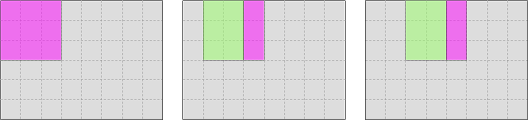
And in the case of output data, the pattern looks like this:

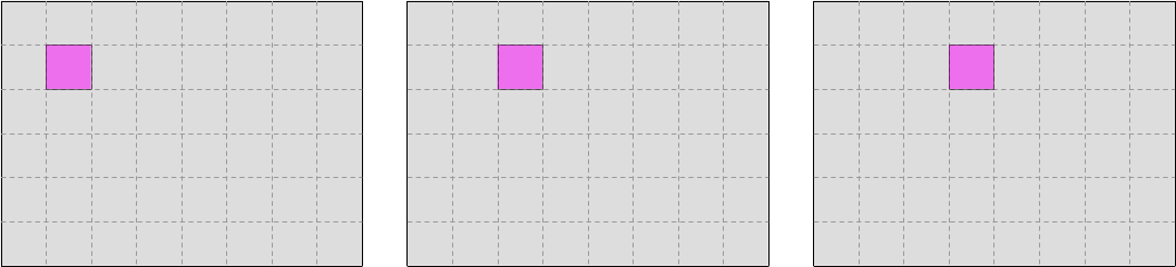
So far so good. As long as we are generating the first row of output data, there is no way to improve upon this pattern. The CPU cache is working as intended, speeding up at least 2/3 of our memory accesses, and it actually helps even more than this when more advanced cache features like hardware prefetching are taken into account.

The question is, what will happen when we reach the second row of output data? Can we reuse the data that we loaded when processing the first row of data, like this?

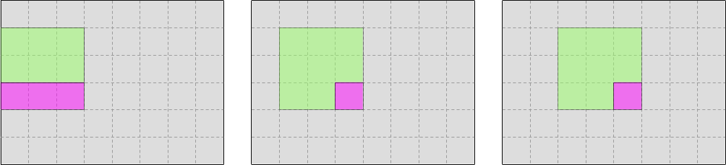
Or do we need to load everything again from RAM or a lower-level cache, like this?

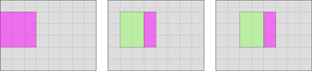
The answer to this question actually depends on how many columns our simulation domain has:

• If the simulation domain has few columns, then by the time we start processing the second row of output, the input data will still be fresh in the L1 CPU cache and can efficiently be reused.
• But if the simulation domain has many columns, by the time we get to the second row, the input data from the beginning of the first row will have been silently dropped by the L1 CPU cache, and we will need to slowly reload it from RAM or a lower-level CPU cache.

We can estimate where the limit lies using relatively simple math:

• Let use denote S the size of the L1 CPU cache in bytes and C the width of the simulation domain in scalar columns.
• In our optimized SIMD data layout, rows of data are padded by 1 SIMD vector of zeros on both sides, so we actually have K = C + 2 * W scalar data columns in our internal tables, where W is our SIMD vector width.
• To produce a row of output, we must read 3 * K data points from the two input tables representing the starting concentrations of species U and V, and we must write K - 2 * W = C data points to the two matching output tables.
• Each data point is a number of type Float, which is currently configured to be of type f32. Therefore, a Float is currently 4 bytes.
• So overall, the CPU cache footprint that is associated while reading input for an entire row is 2 * (3 * K) * 4 = 24 * K bytes and the CPU cache footprint that is associated with writing output for an entire row is 2 * C * 4 = 8 * C bytes.
• By combining these two expressions, it follows that the total CPU cache footprint associated with producing one row of output is 24 * K + 8 * C bytes. Which, if we inject the value of K into the expression, translates into 32 * C + 48 * W bytes.
• For optimal performance, we would like all this data to fit in L1 cache, so that input data is still accessible by the time we start processing the second row, knowing that we need some headroom for other things that go into the L1 cache like constant data. So overall we would like to have 32 * C + 48 * W < S.
• And because we are actually interested in the maximal value of C, we rewrite this expression into the mathematically equivalent C < (S - 48 * W) / 32.

By injecting concrete values of S and W into this expression, we get a maximal value of C for which a given CPU can operate at optimal L1 cache efficiency.

For example, if we consider an Intel i9-10900 CPU with 32 KiB of L1d cache and 256-bit AVX vectors, the limit of L1d cache capacity is reached when the simulation domain has around 976 columns (not accounting for other data which must fit in L1d cache). And unsurprisingly, this does indeed match the point where our microbenchmark’s performance drops.

So far so good, we have a theoretical model that is good enough to model the issue. Let us now use it to improve L1 cache hit rates at larger problem sizes!

The loop blocking trick

So far, we have used a simple iteration scheme where we fully iterate over each row of output concentrations, before moving to the next one:

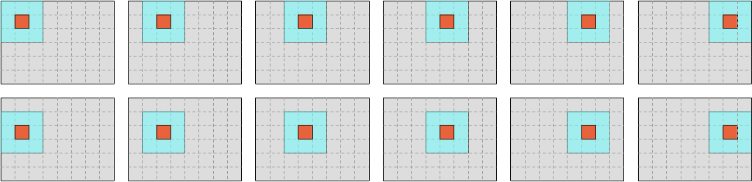
It doesn’t have to be that way however. We could use a different scheme where we slice our data into a number of vertical blocks, and iterate over each vertical block before moving to the next one.

For example, we could first iterate over the left half of the data like this…

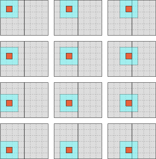
…and then iterate over the right half like this:

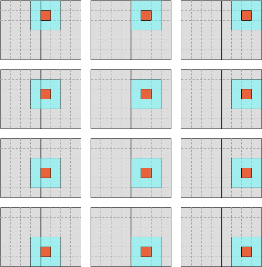
The computation is not sensitive to the order in which data points are computed, so this change of iteration order will not affect the results. What it will do, however, is to reduce the number of columns that are traversed before the computation moves to the next line, ideally ensuring that a large computation which did not fully leverage the CPU’s L1 cache before is now able to do so.

How wide should the blocks be? Well, there is a trade-off there. On one hand, CPUs work best when they are processing long, uninterrupted sequences of contiguous data, and from this perspective longer rows of data are better. On the other hand, the whole point of this chapter is to show you that long row lengths can be problematic for L1d cache locality. Taken together, these two statements entail that we should strive to make our blocks should as wide as available L1d cache capacity will allow, but no wider.

Which is where the simple theoretical model that we derived previously comes into play: using it, we will be able to determine how wide blocks could ideally be, assuming that the L1d cache were fully available for simulation data. We will then shrink this estimate using an empirically tuned safety factor in order to leave some L1d cache headroom for other program state (like constants) and CPU memory subsystem black magic like prefetches. And this is how we will get our optimal block width.

Determining the block width

Recall that our simple theoretical model gives us an C < (S - 48 * W) / 32 bound on block width, where S is the size of the L1d cache and W is our SIMD vector width. We already have seen how one can query the SIMD vector width. But where are we supposed to find out how large the L1d cache is, given that it depends on your CPU, and sometimes even on the core where you are executing?¹

In a C program, the easiest way to query the cache layout of your CPU would be to use the excellent hwloc library, which abstracts over hardware and OS specifics and gives you an easy and portable way to query CPU topology information. But since we are doing Rust, using hwloc directly will involve some unpleasant and unidiomatic unsafe constructs.

Therefore, my recommendation will instead be for you to use hwlocality, a safe binding that I wrote on top of hwloc in order to make it easier to use from Rust.

We start by adding it to our project via a now familiar procedure…²

cargo add hwlocality

And then, inside of our code, we can easily use it to find the minimum L1d cache size across all available CPU cores:

use hwlocality::Topology;

let topology = Topology::new().expect("Failed to query hwloc topology");
let cache_stats = topology
    .cpu_cache_stats()
    .expect("Failed to probe CPU cache stats");
let l1d_size = cache_stats.smallest_data_cache_sizes()[0];

From this, we can deduce an upper bound on the optimal block width…

let l1d_size = smallest_l1d_cache_size();
let float_size = std::mem::size_of::<Float>();
let max_scalar_block_width = (l1d_size as usize - 12 * float_size * simd_width) / (8 * float_size);

…convert it to a number of SIMD vectors to account for our actual data layout…

let max_simd_block_width = max_scalar_block_width / simd_width;

…and shrink it down by a safety factor (that we will late tune through microbenchmarking) in order to account for other uses of the L1d cache that our simple theoretical model does not cover:

// FIXME: Adjust this safety factor through microbenchmarking
let ideal_simd_block_width = (max_simd_block_width as f32 * 0.8) as usize

Putting it all together, we get this function:

/// Determine the optimal block size of the computation
pub fn simd_cols_per_block(simd_width: usize) -> usize {
    let topology = Topology::new().expect("Failed to query hwloc topology");
    let cache_stats = topology
        .cpu_cache_stats()
        .expect("Failed to probe CPU cache stats");
    let l1d_size = cache_stats.smallest_data_cache_sizes()[0];

    let float_size = std::mem::size_of::<Float>();
    let max_scalar_block_width =
        (l1d_size as usize - 12 * float_size * simd_width) / (8 * float_size);
    let max_simd_block_width = max_scalar_block_width / simd_width;

    // FIXME: Adjust this safety factor through microbenchmarking
    (max_simd_block_width as f32 * 0.8) as usize
}

One thing to bear in mind here is that although the code may look innocent enough, computing the block size involves some relatively expensive operations like querying the CPU’s memory subsystem topology from the OS. So we should not do it on every call to the update() function. Instead, it should be computed once during simulation initialization and kept around across update() calls.

Block-wise iteration

Now that we have a block size, let’s slice up our computation domain into actual blocks.

We start by adding a parameter to our update method so that the caller can pass in the precalculated chunk size.

pub fn update<const SIMD_WIDTH: usize>(
    opts: &UpdateOptions,
    start: &UV<SIMD_WIDTH>,
    end: &mut UV<SIMD_WIDTH>,
    cols_per_block: usize,  // <- This is new
) where
    LaneCount<SIMD_WIDTH>: SupportedLaneCount,
{
    // TODO: Implementation
}

Then we extract the center of the output array and we slice it up into non-overlapping chunks:

use ndarray::Axis;

let center_shape = end.simd_shape().map(|dim| dim - 2);
let center = s![1..=center_shape[0], 1..=center_shape[1]];
let mut end_u_center = end.u.slice_mut(center);
let mut end_v_center = end.v.slice_mut(center);
let end_u = end_u_center.axis_chunks_iter_mut(Axis(1), cols_per_block);
let end_v = end_v_center.axis_chunks_iter_mut(Axis(1), cols_per_block);

So far, ndarray makes life easy for us. But unfortunately, it does not have an axis iterator that matches the semantics that we have for input windows, and therefore we are going to need to hack it using careful indexing.

We start by iterating over output blocks, using enumerate() and a counter of blocks to tell when we are going to reach the last block (which may be narrower than the other blocks)..

let num_blocks = center_shape[1].div_ceil(cols_per_block);
for (idx, (end_u, end_v)) in end_u.zip(end_v).enumerate() {
    let is_last = idx == (num_blocks - 1);

    // TODO: Process one output block here
}

…and then we slice up input blocks of the right size:

use ndarray::Slice;

let input_base = idx * cols_per_block;
let input_slice = if is_last {
    Slice::from(input_base..)
} else {
    Slice::from(input_base..input_base + cols_per_block + 2)
};
let start_u = start.u.slice_axis(Axis(1), input_slice);
let start_v = start.v.slice_axis(Axis(1), input_slice);

At this point, we have correctly sized start_u, start_v, end_u and end_v blocks. But our stencil_iter() function cannot accept them yet because the code has so far been specialized to take full UV structs as input, and cannot handle chunks of the simulation domain yet.

I will spare you the required code adjustments since the fine art of generalizing unsafe Rust code without compromizing its safety is beyond the scope of this short course. But in the end we get this:

use ndarray::ArrayViewMut2;

#[inline]
pub fn stencil_iter<'data, const SIMD_WIDTH: usize>(
    start_u: ArrayView2<'data, Vector<SIMD_WIDTH>>,
    start_v: ArrayView2<'data, Vector<SIMD_WIDTH>>,
    mut end_u_center: ArrayViewMut2<'data, Vector<SIMD_WIDTH>>,
    mut end_v_center: ArrayViewMut2<'data, Vector<SIMD_WIDTH>>,
) -> impl Iterator<
    Item = (
        ArrayView2<'data, Vector<SIMD_WIDTH>>, // <- Input u window
        ArrayView2<'data, Vector<SIMD_WIDTH>>, // <- Input v window
        &'data mut Vector<SIMD_WIDTH>,         // <- Output u
        &'data mut Vector<SIMD_WIDTH>,         // <- Output v
    ),
>
where
    LaneCount<SIMD_WIDTH>: SupportedLaneCount,
{
    // Assert that the sub-grids all have the expected memory layout.
    assert_eq!(start_u.shape(), start_v.shape());
    assert_eq!(end_u_center.shape(), end_v_center.shape());
    assert_eq!(start_u.shape().len(), 2);
    assert_eq!(end_u_center.shape().len(), 2);
    assert!(start_u
        .shape()
        .iter()
        .zip(end_u_center.shape())
        .all(|(start_dim, end_dim)| *start_dim == end_dim + 2));
    assert_eq!(start_u.strides(), start_v.strides());
    assert_eq!(start_u.strides(), end_u_center.strides());
    assert_eq!(start_u.strides(), end_v_center.strides());

    // Collect and check common layout information
    let in_shape = [start_u.shape()[0], start_u.shape()[1]];
    assert!(in_shape.into_iter().min().unwrap() >= 2);
    let strides = start_u.strides();
    assert_eq!(strides.len(), 2);
    assert!(strides.iter().all(|stride| *stride > 0));
    let [row_stride, col_stride] = [strides[0] as usize, strides[1] as usize];
    assert_eq!(col_stride, 1);
    let [out_rows, out_cols] = in_shape.map(|dim| dim - 2);

    // Determine how many elements we must skip in order to go from the
    // past-the-end element of one row to the first element of the next row.
    let next_row_step = row_stride - out_cols;

    // Prepare a way to access input windows and output refs by output position
    // The safety of the closures below is actually asserted on the caller's
    // side, but sadly unsafe closures aren't a thing in Rust yet.
    let stencil_shape = [STENCIL_WEIGHTS.len(), STENCIL_WEIGHTS[0].len()];
    let window_shape = (stencil_shape[0], stencil_shape[1]).strides((row_stride, 1));
    let unchecked_output = move |out_ptr: *mut Vector<SIMD_WIDTH>| unsafe { &mut *out_ptr };
    let unchecked_input_window = move |in_ptr: *const Vector<SIMD_WIDTH>| unsafe {
        ArrayView2::from_shape_ptr(window_shape, in_ptr)
    };

    // Recipe to emit the currently selected input windows and output references,
    // then move to the next column. As before, this is only safe if called with
    // correct element pointers.
    let emit_and_increment =
        move |in_u_ptr: &mut *const Vector<SIMD_WIDTH>,
              in_v_ptr: &mut *const Vector<SIMD_WIDTH>,
              out_u_ptr: &mut *mut Vector<SIMD_WIDTH>,
              out_v_ptr: &mut *mut Vector<SIMD_WIDTH>| unsafe {
            let win_u = unchecked_input_window(*in_u_ptr);
            let win_v = unchecked_input_window(*in_v_ptr);
            let out_u = unchecked_output(*out_u_ptr);
            let out_v = unchecked_output(*out_v_ptr);
            *in_u_ptr = in_u_ptr.add(1);
            *in_v_ptr = in_v_ptr.add(1);
            *out_u_ptr = out_u_ptr.add(1);
            *out_v_ptr = out_v_ptr.add(1);
            (win_u, win_v, out_u, out_v)
        };

    // Set up iteration state
    let mut in_u_ptr = start_u.as_ptr();
    let mut in_v_ptr = start_v.as_ptr();
    let mut out_u_ptr = end_u_center.as_mut_ptr();
    let mut out_v_ptr = end_v_center.as_mut_ptr();
    //
    // End of the current row processed by out_v_ptr
    let mut out_v_row_end = unsafe { out_v_ptr.add(out_cols) };
    //
    // End of the last row of the output grid
    let out_v_end = unsafe { out_v_row_end.add(out_rows.saturating_sub(1) * row_stride) };

    // Emit output iterator
    std::iter::from_fn(move || {
        // Common case : we are within the bounds of a row and advance normally
        if out_v_ptr < out_v_row_end {
            return Some(emit_and_increment(
                &mut in_u_ptr,
                &mut in_v_ptr,
                &mut out_u_ptr,
                &mut out_v_ptr,
            ));
        }

        // Otherwise, check if we reached the end of iteration
        if out_v_ptr == out_v_end {
            return None;
        }

        // We're at the end of a row, but not at the end of iteration:
        // switch to the next row then emit the next element as usual
        debug_assert_eq!(out_v_ptr, out_v_row_end);
        unsafe {
            in_u_ptr = in_u_ptr.add(next_row_step);
            in_v_ptr = in_v_ptr.add(next_row_step);
            out_u_ptr = out_u_ptr.add(next_row_step);
            out_v_ptr = out_v_ptr.add(next_row_step);
            out_v_row_end = out_v_ptr.add(out_cols);
        }
        Some(emit_and_increment(
            &mut in_u_ptr,
            &mut in_v_ptr,
            &mut out_u_ptr,
            &mut out_v_ptr,
        ))
    })
}

Basically, where we used to slice the center of the output ourselves, the caller is now responsible for doing it, and the rest is similar as slicing an N-d array does not affect the memory stride from one row to the next, which is the main low-level layout information that we rely on here.

Exercise

Integrate this loop blocking optimization into the code. Note that this will require some changes to the run_simulation function.

Then microbenchmark the code, and adjust the security factor in the implementation of simd_cols_per_block to see how it affects performance. The results may surprise you!³

Parallelism

Well, that last chapter was a disappointment. All this refactoring work, only to find out in the final microbenchmark that the optimization we implemented does improve L1d cache hit rate (as can be measured using perf stat -d), but this improvement in this CPU utilization efficiency metric does not translate into an improvement in execution speed.

The reason is not clear to me at this point in time, unfortunately. It could be several things:

• The CPU manages to hide the latency of L1d cache misses by executing other pending instructions. So even at a 20% L1d cache miss rate we are still not memory-bound.
• The optimization is somehow not implemented properly and costs more than it helps. I have checked for absence of simple issues here, but there could be more subtle ones around.
• There is another, currently unknown factor preventing the execution of more instructions per cycles. So even if data is more readily available in the L1d cache, we still can’t use it yet.

Hopefully I will find the time to clarify this before the next edition of this school. But for now, let us move to the last optimization that should be performed once we are convinced that we are using a single CPU core as efficiently as we can, namely using all of our other CPU cores.

Another layer of loop blocking

There is an old saying that almost every problem in programming can be resolved by adding another layer of indirection. However it could just as well be argued that almost every problem in software performance optimization can be resolved by adding another layer of loop blocking.

In this particular case, the loop blocking that we are going to add revolves around slicing our simulation domain into independent chunks that can be processed by different CPU cores for parallelism. Which begs the question: in which direction should all those chunks be cut? Across rows or columns? And how big should they be?

Let’s start with the first question. We are using ndarray, which in its default configuration stores data in row-major order. And we also know that CPUs are very fond of iterating across data in long linear patterns, and will make you pay a hefty price for any sort of jump across the underlying memory buffer. Therefore, we should think twice before implementing any sort of chunking that makes the rows that we are iterating over shorter, which means that chunking the data into blocks of rows for parallelization is a better move.

As for how big the chunks should be, it is basically a balance between two factors:

• Exposing more opportunities for parallelism and load balancing by cutting smaller chunks. This pushes us towards cutting the problem into at least N chunks where N is the number of CPU cores that our system has, and preferably more to allow for dynamic load balancing of tasks between CPU cores when some cores process work slower than others.¹
• Amortizing the overhead of spawning and awaiting parallel work by cutting larger chunks. This pushes us towards cutting the problem into chunks no smaller than a certain size, dictated by processing speed and task spawning and joining overhead.

The rayon library can take care of the first concern for us by dynamically splitting work as many times as necessary to achieve good load balancing on the specific hardware and system that we’re dealing with at runtime. But as we have seen before, it is not good at enforcing sequential processing cutoffs. Hence we will be taking that matter into our own hands.

Configuring the minimal block size

In the last chapter, we have been using a hardcoded safety factor to pick the number of columns in each block, and you could hopefully see during the exercises that this made the safety factor unpleasant to tune. This chapter will thus introduce you to the superior approach of making the tuning parameters adjustable via CLI parameters and environment variables.

clap makes this very easy. First we enable the environment variable feature…

cargo add --features=env clap

…we add the appropriate option to our UpdateOptions struct…

#[derive(Debug, Args)]
pub struct UpdateOptions {
    // ... unchanged existing options ...

    /// Minimal number of data points processed by a parallel task
    #[arg(env, long, default_value_t = 100)]
    pub min_elems_per_parallel_task: usize,
}

That’s it. Now if we either pass the --min-elems-per-parallel-task option to the simulate binary or set the MIN_ELEMS_PER_PARALLEL_TASK environment variable, that can be used as our sequential processing granularity in the code that we are going to write next.

Adding parallelism

We then begin our parallelism journey by enabling the rayon support of the ndarray crate. This enables some ndarray producers to be turned into Rayon parallel iterators.

cargo add --features=rayon ndarray

Next we split our update() function into two:

• One top-level update() function that will be in charge of receiving user parameters, extracting the center of the output arrays, and parallelizing the work if deemed worthwhile.
• One inner update_seq() function that will do most of the work that we did before, but using array windows instead of manipulating the full concentration arrays directly.

Overall, it looks like this:

/// Parallel simulation update function
pub fn update<const SIMD_WIDTH: usize>(
    opts: &UpdateOptions,
    start: &UV<SIMD_WIDTH>,
    end: &mut UV<SIMD_WIDTH>,
    cols_per_block: usize,
) where
    LaneCount<SIMD_WIDTH>: SupportedLaneCount,
{
    // Extract the center of the output domain
    let center_shape = end.simd_shape().map(|dim| dim - 2);
    let center = s![1..=center_shape[0], 1..=center_shape[1]];
    let mut end_u_center = end.u.slice_mut(center);
    let mut end_v_center = end.v.slice_mut(center);

    // Translate the element-based sequential iteration granularity into a
    // row-based granularity.
    let min_rows_per_task = opts
        .min_elems_per_parallel_task
        .div_ceil(end_u_center.ncols() * SIMD_WIDTH);

    // Run the sequential simulation
    if end_u_center.nrows() > min_rows_per_task {
        // TODO: Run the simulation in parallel
    } else {
        // Run the simulation sequentially
        update_seq(
            opts,
            start.u.view(),
            start.v.view(),
            end_u_center,
            end_v_center,
            cols_per_block,
        );
    }
}

/// Sequential update on a subset of the simulation domain
#[multiversion(targets("x86_64+avx2+fma", "x86_64+avx", "x86_64+sse2"))]
pub fn update_seq<const SIMD_WIDTH: usize>(
    opts: &UpdateOptions,
    start_u: ArrayView2<'_, Vector<SIMD_WIDTH>>,
    start_v: ArrayView2<'_, Vector<SIMD_WIDTH>>,
    mut end_u: ArrayViewMut2<'_, Vector<SIMD_WIDTH>>,
    mut end_v: ArrayViewMut2<'_, Vector<SIMD_WIDTH>>,
    cols_per_block: usize,
) where
    LaneCount<SIMD_WIDTH>: SupportedLaneCount,
{
    // Slice the output domain into vertical blocks for L1d cache locality
    let num_blocks = end_u.ncols().div_ceil(cols_per_block);
    let end_u = end_u.axis_chunks_iter_mut(Axis(1), cols_per_block);
    let end_v = end_v.axis_chunks_iter_mut(Axis(1), cols_per_block);

    // Iterate over output blocks
    for (block_idx, (end_u, end_v)) in end_u.zip(end_v).enumerate() {
        let is_last = block_idx == (num_blocks - 1);

        // Slice up input blocks of the right width
        let input_base = block_idx * cols_per_block;
        let input_slice = if is_last {
            Slice::from(input_base..)
        } else {
            Slice::from(input_base..input_base + cols_per_block + 2)
        };
        let start_u = start_u.slice_axis(Axis(1), input_slice);
        let start_v = start_v.slice_axis(Axis(1), input_slice);

        // Process current input and output blocks
        for (win_u, win_v, out_u, out_v) in stencil_iter(start_u, start_v, end_u, end_v) {
            // TODO: Same code as before
        }
    }
}

Once this is done, parallelizing the loop becomes a simple matter of implementing loop blocking as we did before, but across rows, and iterating over the blocks using Rayon parallel iterators instead of sequential iterators:

// Bring Rayon parallel iteration in scope
use rayon::prelude::*;

// Slice the output domain into horizontal blocks for parallelism
let end_u = end_u_center.axis_chunks_iter_mut(Axis(0), min_rows_per_task);
let end_v = end_v_center.axis_chunks_iter_mut(Axis(0), min_rows_per_task);

// Iterate over parallel tasks
let num_tasks = center_shape[0].div_ceil(min_rows_per_task);
end_u
    .into_par_iter()
    .zip(end_v)
    .enumerate()
    .for_each(|(task_idx, (end_u, end_v))| {
        let is_last_task = task_idx == (num_tasks - 1);

        // Slice up input blocks of the right height
        let input_base = task_idx * min_rows_per_task;
        let input_slice = if is_last_task {
            Slice::from(input_base..)
        } else {
            Slice::from(input_base..input_base + min_rows_per_task + 2)
        };
        let start_u = start.u.slice_axis(Axis(0), input_slice);
        let start_v = start.v.slice_axis(Axis(0), input_slice);

        // Process the current block sequentially
        update_seq(opts, start_u, start_v, end_u, end_v, cols_per_block);
    });

Exercise

Integrate these changes into your codebase, then adjust the available tuning parameters for optimal runtime performance:

• First, adjust the number of threads that rayon uses via the RAYON_NUM_THREADS environment variable. If the machine that you are running on has hyper-threading enabled, it is almost always a bad idea to use it on performance-optimized code, so using half the number of system-reported CPUs will already provide a nice speedup. And since rayon is not NUMA-aware yet, using more threads than the number of cores in one NUMA domain (which you can query using lscpu) may not be worthwhile.
• Next, try to tune the MIN_ELEMS_PER_PARALLEL_TASK parameter. Runtime performance is not very sensitive to this parameter, so you will want to start with big adjustments by factors of 10x more or 10x less, then fine-tune with smaller adjustements once you find a region of the parameter space that seems optimal. Finally, adjust the defaults to your tuned value.

And with that, if we ignore the small wrinkle of cache blocking not yet working in the manner where we would expect it to work (which indicates that there is a bug in either our cache blocking implementation or our expectation of its impact), we have taken Gray-Scott reaction computation performance as far as Rust will let us on CPU.

Stay tuned for next week’s session, where we will see how we to run the computation on a GPU!

From zero to device

In the previous chapters, we have seen how to use Rust to implement an efficient CPU-based simulation of the Gray-Scott reaction. However, these days, CPUs are only half of the story, as most computers also come equipped with one or more GPU(s).

Originally designed for the low-dimensional linear algebra workloads of real-time computer graphics, GPUs have since been remarketed as general-purpose computing hardware, and successfully sold in large numbers to high performance computing centers worldwide. As a result, if you intend to run your computations on HPC centers, you need to know that being able to use a compute node’s GPUs is increasingly becoming a mandatory requirement for larger computing resource allocations.

But even if you don’t care about HPC centers, it is still good to know how to use a GPU for compute, as it is not uncommon for other people to run your code on gaming- or CAD-oriented hardware that has around 10x more single-precision¹ floating-point computing power and RAM bandwidth on the GPU side than on the CPU side.

Therefore, in this part of the course, we will learn how Rust code can be made to leverage almost any available GPU (not just NVidia ones), with minimal end user installation requirements and good portability across operating systems, by leveraging the Vulkan API.

Being fair about Vulkan complexity

Like most other APIs designed by the Khronos Group, Vulkan has a reputation of being very verbose, requiring hundreds of lines of code in order to perform the simplest tasks. While that statement is not wrong, it is arguably incomplete and misleading:

• Vulkan is specified as a C API. This is necessary for it to be callable from many programming languages, but due to limitations of its type system, C tends to make patterns like resource managements and optional features verbose. This is why it is a good idea to avoid using C APIs directly, and instead prefer higher-level language-specific wrappers that leverage the extra capabilities of modern type systems for ergonomics, like vulkano in Rust.
• While a Vulkan “Hello world” is indeed quite long, much of it revolves around one-time initialization work that would not need to be repeated in a larger application. As a consequence, less trivial Vulkan programs will be more comparable in size to programs written against other APIs that have a less flexible initialization process.
• Many lines of the typical Vulkan “Hello world” revolve around things that will not vary much across applications, like enumerating available computing devices and finding out which device you want to use. With a bit of care, these patterns can be easily extracted into libraries of common abstractions, that can easily reuse from one application to another.
• Once all this “accidental verbosity” is taken care of, what remains is extra configuration steps that let you control more details of the execution of your application than is possible in other APIs. This control can be leveraged for performance optimizations, enabling well-written Vulkan applications to use the GPU more efficiently than e.g. CUDA or SYCL applications could.

Keeping these facts in mind, and balancing them against the need to fit this course in half a day and not to make you run away as new learners, this GPU course will mimick the CPU course by providing you with lots of pre-written boilerplate code upfront.

As before, we will spend the next few sections explaining how the provided code works. But because Vulkan programming is a fair bit more complex than CPU programming, here it will actually take not just a few sections, but a few chapters.

Adding the vulkano dependency

First of all, we add vulkano to our list of dependencies. This is a high-level Vulkan binding that will take care of providing an idiomatic Rust interface to the Vulkan C API, and also provide us with a good default policy for handling particularly unpleasant aspects of Vulkan like functionality enumeration², GPU buffer sub-allocation³ and pipeline barriers⁴.

We started by adding the library to our dependencies, as is now customary…

cargo add --optional vulkano

…but this time we made it an optional dependency, which is not built by default, so that your CPU builds are not affected by this relatively heavy dependency.

We then added this dependency to a gpu optional feature inside of the project’s Cargo.toml file:

[features]
gpu = ["dep:vulkano"]

This way, when the project is build with the --features=gpu cargo option, vulkano will be built and linked against our project.

This means that all of our GPU code will more generally need to be guarded so that it is only compiled when this optional feature is enabled. We will later see how that is done.

Loading the Vulkan library

Now that we have vulkano in our dependency tree, we must make it load our operating system’s Vulkan implementation. This is harder than it sounds on the implementation side², but vulkano makes it easy enough for us:

use vulkano::VulkanLibrary;

// Try to load the Vulkan library, and handle errors (here by propagating them)
let library = VulkanLibrary::new()?;

We can then query the resulting VulkanLibrary object in order to know more about the Vulkan implementation that we are dealing with:

• Which version of the Vulkan specification is supported?
• Are there optional extensions that we can enable? These enable us to do things like log driver error messages or display images on the screen.
• Are there optional layers that we can enable? These intercept each of our API calls, typically for the purpose of measuring profiles or validating that our usage of Vulkan is correct.

Creating an instance

Once we have learned everything that we need to know about the Vulkan implementation of the host system, we proceed to create an Instance. This is where we actually initialize the Vulkan library by telling it more about our application and what optional Vulkan functionality it needs.

For this purpose, and many others, vulkano uses a pattern of configuration structs with a default value. You can use the defaults for most fields and set the fields you want differently using the following syntax:

use vulkano::instance::InstanceExtensions;

// Let us log Vulkan errors and warnings
let enabled_extensions = InstanceExtensions {
    ext_debug_utils: true,
    ..Default::default()
};

By using this pattern on a larger scale, we can set up a Vulkan instance that enables minimal debugging functionality (error and warning logging) in release builds, and a more extensive set of debug functionality in debug builds.

use vulkano::instance::{
    Instance, InstanceCreateInfo, InstanceExtensions,
    debug::{
        DebugUtilsMessengerCallback, DebugUtilsMessengerCreateInfo,
        DebugUtilsMessageSeverity, DebugUtilsMessageType
    },
};

// Basic logging in release builds, more logging in debug builds
let mut message_severity =
    DebugUtilsMessageSeverity::ERROR | DebugUtilsMessageSeverity::WARNING;
if cfg!(debug_assertions) {
    message_severity |=
        DebugUtilsMessageSeverity::INFO | DebugUtilsMessageSeverity::VERBOSE;
}
let mut message_type = DebugUtilsMessageType::GENERAL;
if cfg!(debug_assertions) {
    message_type |=
        DebugUtilsMessageType::VALIDATION | DebugUtilsMessageType::PERFORMANCE;
}

// Logging configuration and callback
let messenger_info = DebugUtilsMessengerCreateInfo {
    message_severity,
    message_type,
    // This is unsafe because we promise not to call the Vulkan API
    // inside of this callback
    ..unsafe {
        DebugUtilsMessengerCreateInfo::user_callback(DebugUtilsMessengerCallback::new(
            |severity, ty, data| {
                eprintln!("[{severity:?} {ty:?}] {}", data.message);
            },
        ))
    }
};

// Set up a Vulkan instance
let instance = Instance::new(
    library,
    InstanceCreateInfo {
        // Enable validation layers in debug builds to catch many Vulkan usage bugs
        enabled_layers: if cfg!(debug_assertions) {
            vec![String::from("VK_LAYER_KHRONOS_validation")]
        } else {
            Vec::new()
        },
        // Enable debug utils extension to let us log Vulkan messages
        enabled_extensions: InstanceExtensions {
            ext_debug_utils: true,
            ..Default::default()
        },
        // Set up a first debug utils messenger that logs Vulkan messages during
        // instance initialization and teardown
        debug_utils_messengers: vec![messenger_info],
        ..Default::default()
    }
)?;

Debug logging after instance creation

The debug_utils_messengers field of the InstanceCreateInfo struct only affects how Vulkan errors and warnings are going to be logged during the instance creation and teardown process. For reasons known to the Vulkan specification authors alone, a separate DebugUtilsMessenger must be configured in order to keep logging messages while the application is running.

Of course, they can both use the same configuration, and we can refactor the code accordingly. First we adjust the InstanceCreateInfo to clone the messenger_info struct instead of moving it away…

debug_utils_messengers: vec![messenger_info.clone()],

…and then we create our separate messenger, like this:

use vulkano::instance::debug::DebugUtilsMessenger;

let messenger = DebugUtilsMessenger::new(instance.clone(), messenger_info);

Log messages will only be emitted as long as this object exists, so we will want to keep it around along with other Vulkan state. We’ll get back to this by eventually stashing all useful Vulkan state into a single VulkanContext struct.

There is one more matter that we need to take care of, however: logging on stderr is fundamentally incompatible with displaying ASCII art in the terminal, like the indicatif progress bars that we have been using so far. If a log is printed while the progress bar is on-screen, it will corrupt its display.

indicatif provides us with a tool to handle this, in the form of the ProgressBar::suspend() method. But our debug utils messenger must be configured to use it, which will not be needed in builds without progress bars like our microbenchmarks.

To handle this concern, we pass down a callback to our instance creation function, which receives a string and is in charge of printing it in a manner as appropriate for the current binary…

use std::{panic::RefUnwindSafe, sync::Arc};
use vulkano::{Validated, VulkanError};

fn create_instance(
    // The various trait bounds are used to assert that it is fine for vulkano
    // to move and use our debug callback anywhere, including on another thread
    debug_println: impl Fn(String) + RefUnwindSafe + Send + Sync + 'static
) -> Result<(Arc<Instance>, DebugUtilsMessenger), Box<dyn Error>> {
    // TODO: Create the instance and its debug messenger
}

…and we use it in our Vulkan logging callback instead of calling eprintln!() directly:

..unsafe {
    DebugUtilsMessengerCreateInfo::user_callback(DebugUtilsMessengerCallback::new(
        move |severity, ty, data| {
            let message = format!("[{severity:?} {ty:?}] {}", data.message);
            debug_println(message);
        },
    ))
}

We will provide a version of this callback that directly sends logs to stderr…

#![allow(unused)]
fn main() {
pub fn debug_println_stderr(log: String) {
    eprintln!("{log}");
}
}

…and a recipe to make other callbacks that use the suspend method of an indicatif ProgressBar to correctly print out logs when such a progress bar is active:

use indicatif::ProgressBar;

pub fn make_debug_println_indicatif(
    progress_bar: ProgressBar
) -> impl Fn(String) + RefUnwindSafe + Send + Sync + 'static {
    move |log| progress_bar.suspend(|| eprintln!("{log}"))
}

To conclude this instance creation tour, let’s explain the return type of create_instance():

Result<(Arc<Instance>, DebugUtilsMessenger), Box<dyn Error>>

There are two layers there:

• We have a Result, which indicates that the function may fail in a manner that the caller can recover from, or report in a customized fashion.
• In case of success, we return an Instance, wrapped in an Arc Atomically Reference-Counted pointer so that cheap copies can be shared around, including across threads⁵.
• In case of error, we return Box<dyn Error>, which is the lazy person’s type for “any error can happen, I don’t care about enumerating them in the output type”.

And that’s finally it for Vulkan instance creation!

Picking a physical device

People who are used to CUDA or SYCL may be surprised to learn that Vulkan works on all modern⁶ GPUs with no other setup work needed than having a working OS driver, and can be easily emulated on CPU for purposes like unit testing in CI.

There is a flip side to this portability, however, which is that it is very common to have multiple Vulkan devices available on a given system, and production-grade code should ideally be able to…

• Tell which of the available devices (if any) match its hardware requirements (e.g. amount of RAM required for execution, desired Vulkan spec version/extensions…).
• If only a single device is to be used⁷, pick the most suitable device amongst those available options (which may involve various trade-offs like peak performance vs power efficiency).

We will at first do the simplest thing that should work on most machines⁸: accept all devices, priorize them by type (discrete GPU, integrated GPU, CPU-based emulation…) according to expected peak throughput, and pick the first device that matches in this priority order.

But as we move forward through the course, we may have to revisit this part of the code by filtering out devices that do not implement certain optional features that we need. Hence we should plan ahead by having a device filtering callback that tells whether each device can be used or not, using the same logic as Iterator::filter().

Finally, we need to decide what will happen if we fail to detect a suitable GPU device. In production-quality code, the right thing to do here would be to log a warning and fall back to a CPU-based computation. And if we have such a CPU fallback available, we should probably also ignore CPU emulations of GPU devices, which are likely to be slower. But because the goal is to learn about how to write Vulkan code here, we will instead fail with a runtime panic when no GPU or GPU emulation is found, as this will tell us if something is wrong with our device selection callback.

Overall, our physical device selection code looks like this:

use vulkano::{
    device::physical::{PhysicalDevice, PhysicalDeviceType},
    VulkanError,
};

/// Pick the best physical device that matches our requirements
fn pick_physical_device(
    instance: &Arc<Instance>,
    mut device_filter: impl FnMut(&PhysicalDevice) -> bool,
) -> Result<Arc<PhysicalDevice>, VulkanError> {
    Ok(instance
        .enumerate_physical_devices()?
        .filter(|device| device_filter(&device))
        .fold(None, |best_so_far, current| {
            // The first device that comes up is always the best
            let Some(best_so_far) = best_so_far else {
                return Some(current);
            };

            // Compare previous best device type to current device type
            let best_device = match (
                best_so_far.properties().device_type,
                current.properties().device_type,
            ) {
                // Discrete GPU should always be the best performing option
                (PhysicalDeviceType::DiscreteGpu, _) => best_so_far,
                (_, PhysicalDeviceType::DiscreteGpu) => current,
                // Virtual GPU is hopefully a discrete GPU accessed via PCIe passthrough
                (PhysicalDeviceType::VirtualGpu, _) => best_so_far,
                (_, PhysicalDeviceType::VirtualGpu) => current,
                // Integrated GPU is, at least, still a GPU.
                // It will likely be less performant, but more power-efficient.
                // In this basic codebase, we'll only care about performance.
                (PhysicalDeviceType::IntegratedGpu, _) => best_so_far,
                (_, PhysicalDeviceType::IntegratedGpu) => current,
                // CPU emulation is probably going to be pretty bad...
                (PhysicalDeviceType::Cpu, _) => best_so_far,
                (_, PhysicalDeviceType::Cpu) => current,
                // ...but at least we know what we're dealing with, unlike the rest
                (PhysicalDeviceType::Other, _) => best_so_far,
                (_, PhysicalDeviceType::Other) => current,
                (_unknown, _other_unknown) => best_so_far,
            };
            Some(best_device)
        })
        // This part (and the function return type) would change if you wanted
        // to switch to a CPU fallback when no GPU is found.
        .expect("No usable Vulkan device found"))
}

Creating a logical device and command queue

Once we have found a suitable physical device, we need to set up a logical device, which will be used to allocate resources. And we will also need to set up with one or more command queues, which will be used to submit work. Both of these will be created in a single API transaction.

The process of creating a logical device and associated command queues is very similar to that of creating a Vulkan instance, and exists partially for the same reasons: we need to pick which optional API features we want to enable, at the expense of reducing application portability.

But here there is also a new concern, which is command queue creation. In a nutshell, Vulkan devices support simultaneous submission and processing of commands over multiple independent hardware channels, which is typically used to…

• Overlap graphics rendering with general-purpose computing.
• Overlap PCIe data transfers to and from the GPU with other operations.

Some channels are specialized for a specific type of operations, and may perform them better than other channels. Unlike most other GPU APIs, Vulkan exposes this hardware feature in the form of queue families with flags that tell you what each family can do. For example, here are the queue families available on my laptop’s AMD Radeon 5600M GPU, as reported by vulkaninfo:

VkQueueFamilyProperties:
========================
    queueProperties[0]:
    -------------------
        minImageTransferGranularity = (1,1,1)
        queueCount                  = 1
        queueFlags                  = QUEUE_GRAPHICS_BIT | QUEUE_COMPUTE_BIT | QUEUE_TRANSFER_BIT
        timestampValidBits          = 64
        present support             = true
        VkQueueFamilyGlobalPriorityPropertiesKHR:
        -----------------------------------------
            priorityCount  = 4
            priorities: count = 4
                QUEUE_GLOBAL_PRIORITY_LOW_KHR
                QUEUE_GLOBAL_PRIORITY_MEDIUM_KHR
                QUEUE_GLOBAL_PRIORITY_HIGH_KHR
                QUEUE_GLOBAL_PRIORITY_REALTIME_KHR


    queueProperties[1]:
    -------------------
        minImageTransferGranularity = (1,1,1)
        queueCount                  = 4
        queueFlags                  = QUEUE_COMPUTE_BIT | QUEUE_TRANSFER_BIT
        timestampValidBits          = 64
        present support             = true
        VkQueueFamilyGlobalPriorityPropertiesKHR:
        -----------------------------------------
            priorityCount  = 4
            priorities: count = 4
                QUEUE_GLOBAL_PRIORITY_LOW_KHR
                QUEUE_GLOBAL_PRIORITY_MEDIUM_KHR
                QUEUE_GLOBAL_PRIORITY_HIGH_KHR
                QUEUE_GLOBAL_PRIORITY_REALTIME_KHR


    queueProperties[2]:
    -------------------
        minImageTransferGranularity = (1,1,1)
        queueCount                  = 1
        queueFlags                  = QUEUE_SPARSE_BINDING_BIT
        timestampValidBits          = 64
        present support             = false
        VkQueueFamilyGlobalPriorityPropertiesKHR:
        -----------------------------------------
            priorityCount  = 4
            priorities: count = 4
                QUEUE_GLOBAL_PRIORITY_LOW_KHR
                QUEUE_GLOBAL_PRIORITY_MEDIUM_KHR
                QUEUE_GLOBAL_PRIORITY_HIGH_KHR
                QUEUE_GLOBAL_PRIORITY_REALTIME_KHR

As you can see, there is one general-purpose queue family that can do everything, another queue family that is specialized for asynchronous compute tasks and data transfers running in parallel with the main compute/graphics work, and a third queue family that lets you manipulate sparse memory resources for the purpose of handling resources larger than GPU VRAM less badly.

From these physical queue families, you may then allocate one or more logical command queues that will allow you to submit commands to the matching hardware command processor.

To keep this introductory course simpler, and because the Gray-Scott reaction simulation does not easily lend itself to the parallel execution of compute and data transfer commands⁹, we will not use multiple command queues in this course. Instead, we will always use a single command queue from the first queue family that supports general-purpose computations and data transfers:

use vulkano::device::QueueFlags;

// Pick the first queue family that supports compute
let queue_family_index = physical_device
    .queue_family_properties()
    .iter()
    .position(|properties| {
        properties
            .queue_flags
            .contains(QueueFlags::COMPUTE | QueueFlags::TRANSFER)
    })
    .expect("Vulkan spec mandates availability of at least one compute queue");

As for optional device features, for now we will…

• Only enable features that are useful for debugging (basically turning out-of-bounds data access UB into well-defined behavior)
• Only do so in debug builds as they may come at a runtime performance cost.
• Only enable them if supported by the device, ignoring their absence otherwise.

Overall, it looks like this:

use vulkano::device::Features;

// Enable debug features in debug builds, if supported by the device
let supported_features = physical_device.supported_features();
let enabled_features = if cfg!(debug_assertions) {
    Features {
        robust_buffer_access: supported_features.robust_buffer_access,
        robust_buffer_access2: supported_features.robust_buffer_access2,
        robust_image_access: supported_features.robust_image_access,
        robust_image_access2: supported_features.robust_image_access2,
        ..Default::default()
    }
} else {
    Features::default()
};

Now that we know which optional features we want to enable and which command queues we want to use, all that is left to do is to create our logical device and single commande queue:

use vulkano::device::{Device, DeviceCreateInfo, QueueCreateInfo};

// Create our device and command queue
let (device, mut queues) = Device::new(
    physical_device,
    DeviceCreateInfo {
        // Request a single command queue from the previously selected family
        queue_create_infos: vec![QueueCreateInfo {
            queue_family_index: queue_family_index as u32,
            ..Default::default()
        }],
        enabled_features,
        ..Default::default()
    },
)?;
let queue = queues
    .next()
    .expect("We asked for one queue, we should get one");

And that concludes our create_device_and_queue() function, which itself is the last part of the basic application setup work that we will always need no matter what we want to do with Vulkan.

In the next chapter, we will see a few more Vulkan setup steps that are a tiny bit more specific to this application, but could still be reused across many different applications.

From device to context

At far as the Vulkan C API is concerned, once we have a device and a queue, we can use pretty much every part of Vulkan. But on a more practical level, there are some extra conveniences that we will want to set up now in order to make our later work easier, and as a practical matter the vulkano high-level API forces us to set up pretty much all of them anyway. These include…

• Sub-allocators, which let us perform fewer larger allocations from the GPU driver¹, and slice them up into the small API objects that we need.
• Pipeline caches, which allow us not to recompile the GPU-side code when neither the code nor the GPU driver has changed. This makes our application run faster, because in GPU applications a large part of the GPU-side compilation work is done at runtime.

We will take care of this remaining vulkano initialization work in this chapter.

Allocators

There are three kinds of objects that a Vulkan program may need to allocate in large numbers:

• Memory objects, like buffers and images. These will contain most of the application data that we are directly interested in processing.
• Command buffer objects. These are used to store batches of GPU commands, that will then be sent to the GPU in order to ask it to do something: transfer data, execute our GPU code…
• Descriptor set objects. These are used to attach a set of memory objects to a GPU program. The reason why Vulkan has them instead of making you bind memory objects to GPU programs one by one is that it allows the binding process to be more CPU-efficient, which matters in applications with short-running GPU programs that have many inputs and outputs.

These objects have very different characteristics (memory footprint, alignment, lifetime, CPU-side access patterns…), and therefore benefit from each having their own specialized allocation logic. Accordingly, vulkano provides us with three standard allocators:

• StandardMemoryAllocator for memory objects
• StandardCommandBufferAllocator for command buffers
• StandardDescriptorSetAllocator for descriptor sets

As the Standard naming implies, these allocators are intended to be good enough for most applications, and easily replaceable when they don’t fit. I can tell you from experience that we are very unlikely to ever need to replace them for our Gray-Scott simulation, so we can just have a couple of type aliases as a minimal future proofing measure…

pub type MemoryAllocator = vulkano::memory::allocator::StandardMemoryAllocator;
pub type CommandBufferAllocator =
    vulkano::command_buffer::allocator::StandardCommandBufferAllocator;
pub type DescriptorSetAllocator =
    vulkano::descriptor_set::allocator::StandardDescriptorSetAllocator;

…and a common initialization function that sets up all of them, using the default configuration as it fits the needs of the Gray-Scott simulation very well.

use std::sync::Arc;
use vulkano::{
    command_buffer::allocator::StandardCommandBufferAllocatorCreateInfo,
    descriptor_set::allocator::StandardDescriptorSetAllocatorCreateInfo,
};

fn create_allocators(
    device: Arc<Device>,
) -> (
    Arc<MemoryAllocator>,
    Arc<CommandBufferAllocator>,
    Arc<DescriptorSetAllocator>,
) {
    let malloc = Arc::new(MemoryAllocator::new_default(device.clone()));
    let calloc = Arc::new(CommandBufferAllocator::new(
        device.clone(),
        StandardCommandBufferAllocatorCreateInfo::default(),
    ));
    let dalloc = Arc::new(DescriptorSetAllocator::new(
        device.clone(),
        StandardDescriptorSetAllocatorCreateInfo::default(),
    ));
    (malloc, calloc, dalloc)
}

You may reasonably wonder why we need to manually wrap the allocators in an Arc atomically reference-counted smart pointer, when almost every other API in vulkano returns an Arc for you. This bad API originates from the fact that vulkano is currently reworking the API of its memory allocators, and had to release v0.34 in the middle of that rework due to user pressure. So things will hopefully improve in the next vulkano release.

Pipeline cache

Why it exists

GPU programs (also called shaders by graphics programmers and kernels by compute programmers) tend to have a more complex compilation process than CPU programs for a few reasons:

• At the time where you compile your application, you generally don’t know what GPU it is eventually going to run on. Needing to recompile the code anytime you want to run on a different GPU, either on the same multi-GPU machine or on a different machine, is a nuisance that many wise people would like to avoid.
• Compared to CPU manufacturers, GPU manufacturers are a lot less attached to the idea of having open ISA specifications. They would rather not fully disclose how their hardware ISA works, and instead only make you manipulate it through a lawyer-approved abstraction layer, that leaks less (presumed) trade secrets and allows them to transparently change more of their hardware architecture from one generation of hardware to the next.
• Because this abstraction layer is fully managed by the GPU driver, the translation of a given program in the fake manufacturer ISA to the actual hardware ISA is not fixed in time and can change from one version of the GPU driver to ther other, as new optimizations are discovered.

Because of this, ahead-of-time compilation of GPU code to the true hardware ISA pretty much does not exist. Instead, some degree of just-in-time compilation is always used. And with that comes the question of how much time you application can spend recompiling the GPU code on every run.

Vulkan approaches this problem from two angles:

• First of all, your GPU code is translated during application compilation into an intermediate representation called SPIR-V, which is derived from LLVM IR. The Vulkan implementation is then specified in terms of SPIR-V. This has several advantages:
  • Hardware vendors, who are not reknowned for their compilation expertise, do not need to manipulate higher-level languages like C anymore. Compared with earlier GPU APIs which trusted them at this, this is a major improvement in GPU driver reliability.
  • Some of the compilation and optimization work can be done at application compilation time. This reduces the amount of work that the GPU driver’s compiler needs to do at application runtime, and the variability of application performance across GPU drivers.
• Second, the result of translating the SPIR-V code to hardware-specific machine code can be saved into a cache and reused in later application runs. For reasons that will become clear later in this course, this cache is called a pipeline cache.

Now, one problem with caches is that they can be invalidated through changes in hardware or GPU driver versions. But Vulkan fully manages this for you. What is left up to you, however, is the work of saving this cache to disk when an application terminates, and reloading it on the next run of the application. Basically, you get a bunch of bytes from Vulkan, and Vulkan entrusts you for somehow saving those bytes somewhere and giving them back unchanged on the next application run.

The point of exposing this process to the application, instead of hiding it like earlier GPU APIs did, is that it gives advanced Vulkan applications power to…

• Invalidate the cache themselves when the Vulkan driver has a bug which leads to cache invalidation failure or corruption.²
• Provide pre-packaged caches for all common GPU drivers so that even the first run of an application is likely to be fast, without JiT compilation of GPU code.

How we handle it

In our case, we will not do anything fancy with the Vulkan pipeline cache, just mimick what other GPU APIs do under the hood by saving it in the operating system’s standard cache directory at application teardown time and loading it back if it exists at application startup time.

First of all, we need to know what the operating system’s standard cache directory location is. Annoyingly, it is very much non-obvious, changes from one OS to another, and varied across the history of each OS. But thankfully there’s a crate/library for that.

First we add it as an optional dependency…

cargo add --optional directories

…and within the project’s Cargo.toml, we make it part of our gpu optional feature.

[features]
gpu = ["dep:directories", "dep:vulkano"]

We then use directories to locate the OS’ standard application data storage directories:

use directories::ProjectsDirs;

let dirs = ProjectDirs::from("", "", "grayscott")
                       .expect("Could not find home directory");

For this simple application, we handle weird OS configurations where the user’s home directory cannot be found by panicking. A more sophisticated application might decide instead not to cache GPU pipelines in this case, or even get dangerous and try random hardcoded paths like /var/grayscott.cache just in case they work out.

Finally, we use the computed directories to make a simple abstraction for cache persistence:

use std::path::PathBuf;
use vulkano::pipeline::cache::{PipelineCache, PipelineCacheCreateInfo};

/// Simple cache management abstraction
pub struct PersistentPipelineCache {
    /// Standard OS data directories for this project: cache, config, etc
    dirs: ProjectDirs,

    /// Vulkan pipeline cache
    pub cache: Arc<PipelineCache>,
}
//
impl PersistentPipelineCache {
    /// Set up a pipeline cache, integrating previously cached data
    fn new(device: Arc<Device>) -> Result<Self, Validated<VulkanError>> {
        // Find standard OS directories
        let dirs = ProjectDirs::from("", "", "grayscott")
                               .expect("Could not find home directory");

        // Try to load former cache data, use empty data on vectors
        let initial_data = std::fs::read(Self::cache_path(&dirs)).unwrap_or_default();

        // Build Vulkan pipeline cache
        //
        // This is unsafe because we solemny promise to Vulkan that we did not
        // fiddle with the bytes of the cache. And since this is GPU vendor
        // code, you better not expect it to validate its inputs.
        let cache = unsafe {
            PipelineCache::new(
                device,
                PipelineCacheCreateInfo {
                    initial_data,
                    ..Default::default()
                },
            )?
        };
        Ok(Self { dirs, cache })
    }

    /// Save the pipeline cache
    ///
    /// It is recommended to call this method manually, rather than let the
    /// destructor save the cache automatically, as this lets you control how
    /// errors are reported and integrate it into a broader application-wide
    /// error handling policy.
    pub fn try_save(&mut self) -> Result<(), Box<dyn Error>> {
        std::fs::write(Self::cache_path(&self.dirs), self.cache.get_data()?)?;
        Ok(())
    }

    /// Compute the pipeline cache path
    fn cache_path(dirs: &ProjectDirs) -> PathBuf {
        dirs.cache_dir().join("PipelineCache.bin")
    }
}
//
impl Drop for PersistentPipelineCache {
    fn drop(&mut self) {
        // Cannot cleanly report errors in destructors
        if let Err(e) = self.try_save() {
            eprintln!("Failed to save Vulkan pipeline cache: {e}");
        }
    }
}

Putting it all together

As you can see, setting up Vulkan involves a number of steps. In computer graphics, the tradition is to regroup all of these steps into the constructor of a large Context struct whose members feature all API objects that we envision to need later on. We will follow this tradition:

pub struct VulkanContext {
    /// Logical device (used for resource allocation)
    pub device: Arc<Device>,

    /// Command queue (used for command submission)
    pub queue: Arc<Queue>,

    /// Memory object allocator
    pub memory_alloc: Arc<MemoryAllocator>,

    /// Command buffer allocator
    pub command_alloc: Arc<CommandBufferAllocator>,

    /// Descriptor set allocator
    pub descriptor_alloc: Arc<DescriptorSetAllocator>,

    /// Pipeline cache with on-disk persistence
    pub pipeline_cache: PersistentPipelineCache,

    /// Messenger that prints out Vulkan debug messages until destroyed
    _messenger: DebugUtilsMessenger,
}
//
impl VulkanContext {
    /// Set up the Vulkan context
    pub fn new(
        debug_println: impl Fn(String) + RefUnwindSafe + Send + Sync + 'static,
    ) -> Result<Self, Box<dyn Error>> {
        let (instance, messenger) = create_instance(debug_println)?;
        // Not imposing any extra constraint on devices for now
        let physical_device = pick_physical_device(&instance, |_device| true)?;
        let (device, queue) = create_device_and_queue(physical_device)?;
        let (memory_alloc, command_alloc, descriptor_alloc) = create_allocators(device.clone());
        let pipeline_cache = PersistentPipelineCache::new(device.clone())?;
        Ok(Self {
            device,
            queue,
            memory_alloc,
            command_alloc,
            descriptor_alloc,
            pipeline_cache,
            _messenger: messenger,
        })
    }

    /// Run all inner manual destructors
    pub fn finish(&mut self) -> Result<(), Box<dyn Error>> {
        self.pipeline_cache.try_save()?;
        Ok(())
    }
}

And with that, we have wrapped up what the gpu::context module of the provided course skeleton does. The rest will be integrated next!

Exercise

In the Rust project that you have been working on so far, the above GPU support is already present, but it is in a dedicated gpu module that is only compiled in when the gpu compile-time feature is enabled. This is achieved using a #[cfg(feature = "gpu")] compiler directive.

So far, that build feature has been disabled by default. This allowed you to enjoy faster builds, unpolluted by the cost of building GPU dependencies like vulkano. These are huge libraries with a significant compilation cost, because Vulkan itself is a huge specification.

However, now that we actually do want to run with GPU support enabled, the default of not building the GPU code is not the right one anymore. Therefore, please add the following line to the [features] section of the Cargo.toml file at the root of the repository:

default = ["gpu"]

This has the same effect as passing --features=gpu to every cargo command that you will subsequently run: it will enable the optional gpu compile-time feature of the project, along with associated optional dependencies.

You will then want to add a VulkanContext::new() call at the beginning of the simulate microbenchmark and binary, call the finish() method.

In the microbenchmark, you will want to handle errors by panicking: just call the expect() method of the output Results with an error message. In bin/simulate, you may instead propagate the errors out of main by switching to the more general result type Result<(), Box<dyn Error>>.

If you have done everything right, both binaries should now compile and run successfully. They are not doing anything useful with Vulkan right now, but lack of error means that our GPU driver/emulation works perform the basic setup work as expected, which is already a start!

Shader

So far, we have mostly been working on common Vulkan boilerplate that could easily be reused in another application, with minor changes and extra configuration options. Now it’s time to actually start writing some Gray-Scott reaction simulation code.

In this chapter, we will write the part of the simulation code that actually runs on the GPU. Vulkan calls it a shader, but if you feel more comfortable calling it a kernel, I won’t judge you. I’ll let the Linux contributors in the room do it for me. 😉

Introducing GLSL

One benefit of Khronos’ decision to switch to the SPIR-V intermediate representation was that it became theoretically possible to use any compiled programming language you like to write the GPU-side code. All you need is a new compiler backend that emits SPIR-V instead of machine code.

Sadly, compiler backends are big pieces of work, so Rust is not quite there yet. All we have today is a promising prototype around called rust-gpu. I hope to introduce it in a future edition of this course¹, but what I read in its bugtracker, it felt a bit too experimental for this year’s edition.

Therefore, we will prefer the tried and true alternative of Khronos’ standard GPU programming language: the OpenGL Shading Language, or GLSL for short.

GLSL is, along with HLSL, one of the two most important programming languages in the history of GPU computing. It was originally designed as a companion to the OpenGL GPU API, the predecessor to Vulkan in Khronos’ family of GPU APIs, and therefore its specification can be found right next to the OpenGL specification on the Khronos Group website.

GLSL is a derivative of the C programming language, which dropped some of C’s most controversial features² and introduced many extensions to C to meet the needs of GPU computing.

To give some examples, in GLSL you can easily…

• Specify how the GPU code will interface with Vulkan on the CPU side.
• Easily manipulate vectors and matrices, but only up to dimension 4x4.³
• Exploit GPU texturing units to more efficiently manipulate 2/3D arrays, interpolate 1/2/3D data, and perform on-the-fly conversions between many image formats.
• Selectively let the compiler optimize operations in a numerically unstable fashion (similar to GCC’s -ffast-math, except SPIR-V makes it fine-grained and calls it RelaxedPrecision).
• Control the fashion in which the GPU program execution’s will be decomposed into work-groups (the Vulkan equivalent of NVidia CUDA’s thread blocks).
• Allow the value of a compilation constant to be specified before the shader’s SPIR-V is compiled into a device binary, to improve configurability and compiler optimizations.
• A more extensive library of built-in functions than C could ever dream of.
• …and many other things revolving around the high-speed drawing of textured triangles that we will not care much about in everyday numerical computing.⁴

As you can see, this opens quite a few interesting possibilities. And that’s part of why rust-gpu is still experimental in spite of having been in development for quite a while. Making a new GPU programming language is actually not only a matter of adding a SPIR-V backend to the compiler (which is already quite a piece of work), it’s also a matter of extending the source programming language (possibly via a library of functions implemented in SPIR-V “assembly”) to expose all the GPU features that GPU-specific programming languages have been supporting forever.⁵

Our first GLSL Gray-Scott

Let us now go through a GLSL implementation of the Gray-Scott reaction simulation. This first implementation isn’t heavily tuned for performance, however it does try to leverage GLSL-specific features where the impact on readability is small and it should help runtime performance.

First of all, we specify which version of the GLSL specification the program is written against. Here, we are using the latest and greatest GLSL 4.60 specification.

#version 460

Then we start to specify the interface between the CPU and the GPU code. This is a danger zone. Anytime we change this part of the GPU code, we must remember to keep matching code on the CPU side in sync, or else the GPU program will produce completely wrong results if it runs at all.

// Initial concentrations of species U and V
layout(set = 0, binding = 0) uniform sampler2D us;
layout(set = 0, binding = 1) uniform sampler2D vs;

// Final concentrations of species U and V
layout(set = 0, binding = 2) uniform restrict writeonly image2D nextUs;
layout(set = 0, binding = 3) uniform restrict writeonly image2D nextVs;

// Computation parameters uniform
layout(set = 1, binding = 0) uniform Parameters {
    mat3 weights;
    float diffusion_rate_u, diffusion_rate_v,
          feed_rate, kill_rate,
          time_step;
} params;

// Workgroup dimensions
layout(local_size_x = 8, local_size_y = 8) in;

There is a fair bit to unpack here:

• us and vs are 2D samplers representing our input data. There are two interfaces to GPU texturing units in Khronos APIs, images and samplers. Images let us leverage the optimized data layout of GPU textures for 2/3D spatial locality. Samplers build on top of images to provide us with optional interpolation features (not used here) and well-defined handling of out-of-bound accesses (used here to enforce the simulation’s zero boundary condition).
• nextUs and nextVs are 2D images representing our output data. Here we do not need samplers because we will not be performing out-of-bounds accesses on the output side. We can also help the GPU compiler optimize code better that telling it that these images do not alias with any other input/output data in memory and will not be read from.
• params is a struct that lets us pass simulation parameters to the GPU code. Notice that unlike the CPU code, the GPU code does not know about some computation parameters at compile time, which puts it at a slight performance disadvantage. By using specialization constants, we could reverse this situation and let the GPU compiler know about all simulation parameters at compile time using specialization constants.
• All variables introduced so far are uniforms, which means that all work-items (same thing as CUDA threads) in a given shader execution agree on their value. This greatly improves GPU code performance by letting the GPU hardware share associated state (registers, etc) between concurrent computations, and is in fact mandatory for images and samplers.
• To enable binding associated resources from the CPU side, each of these inputs and outputs is assigned a set and binding number. Here, we have made all inputs and outputs part of set 0, and parameters part of set 1. Here the two layer set->binding hierarchy lets us flip simulation inputs and outputs without needing to rebind unchanging simulation parameters.
• Finally, we specify the work-group size, which is Vulkan’s equivalent of CUDA’s thread-block size. For now, we hardcode it in the shader code, but later we can make it runtime-configurable using specialization constants.

After specifying the CPU/GPU interface, we add a few simple utilities to make it easier to use. First, we write a pair of more ergonomic wrappers on top of GLSL’s very general but somewhat unwieldy image and sampler access functions…

// Read the current value of the concentration
vec2 read_uv(const ivec2 input_idx) {
    const vec2 input_pos = vec2(input_idx) + 0.5;
    return vec2(
        texture(us, input_pos).r,
        texture(vs, input_pos).r
    );
}

// Write the next value of the concentration
void write_uv(const ivec2 output_idx, const vec2 uv) {
    imageStore(nextUs, output_idx, vec4(uv.x));
    imageStore(nextVs, output_idx, vec4(uv.y));
}

…and second, we give ourselves a way to refer to the stencil’s 2D dimensions and center position:

// Diffusion stencil properties
const ivec2 stencil_shape = ivec2(params.weights.length(),
                                  params.weights[0].length());
const ivec2 stencil_offset = ivec2((stencil_shape - 1) / 2);

Finally, we introduce the body of the Gray-Scott reaction computation:

// What each shader invocation does
void main() {
    // Determine which central input and output location we act on
    const ivec2 center_idx = ivec2(gl_GlobalInvocationID.xy);

    // Read the center value of the concentration
    const vec2 uv = read_uv(center_idx);

    // Compute diffusion term for U and V
    vec2 full_uv = vec2(0.);
    const ivec2 top_left = center_idx - stencil_offset;
    for (int x = 0; x < stencil_shape.x; ++x) {
        for (int y = 0; y < stencil_shape.y; ++y) {
            const vec2 stencil_uv = read_uv(top_left + ivec2(x, y));
            full_uv += params.weights[x][y] * (stencil_uv - uv);
        }
    }
    const float diffusion_u = params.diffusion_rate_u * full_uv.x;
    const float diffusion_v = params.diffusion_rate_v * full_uv.y;

    // Deduce rate of change in u and v
    const float u = uv.x;
    const float v = uv.y;
    const float uv_square = u * v * v;
    const float du = diffusion_u - uv_square + params.feed_rate * (1.0 - u);
    const float dv = diffusion_v + uv_square
                                 - (params.feed_rate + params.kill_rate) * v;

    // Update u and v accordingly
    write_uv(center_idx, uv + vec2(du, dv) * params.time_step);
}

Again, this could use some unpacking:

• Like CUDA, Vulkan and GLSL use a data-parallel execution model where each work-item is tasked with processing one element of a 1/2/3D-dimensional grid. We can read the position that we are tasked to process from the gl_GlobalInvocationID global 3D vector. Because our problem is 2D, we extract the first two coordinates of this vector, and convert them from floating-point to integer because that feels most correct here.
• We then compute the diffusion term of the differential equation. Here we played a little with GLSL’s vector type to make the computations of U and V less redundant and possibly a little more efficient (depending on how smart your GPU driver’s compiler feels like being today).
• Finally, we update U and V using almost exactly the same logic as the CPU version.

Basic CPU-side integration

Following the historical conventions of GPU programmers, we first save our GPU-side code into a source file with a .comp extension, which tells our IDE tooling that this is a compute shader. We propose that you call it grayscott.comp and put it inside of the exercises/src/gpu.

We then ensure that this shader is compiled to SPIR-V whenever our project is built by using the vulkano-shaders library provided by the vulkano project. We first add it as a dependency…

cargo add --optional vulkano-shaders

…and within the project’s Cargo.toml, we make it part of our gpu optional feature.

[features]
gpu = ["dep:directories", "dep:vulkano", "dep:vulkano-shaders"]

Then within our code’s gpu::pipeline module, we create a new shader module and ask vulkano_shaders to generate the SPIR-V code and some Rust support code inside of it:

/// Compute shader used for GPU-side simulation
mod shader {
    vulkano_shaders::shader! {
        ty: "compute",
        path: "src/gpu/grayscott.comp",
    }
}

Finally, to make the code more maintainable, we give human-readable names to the shader binding points. These constants will still need to be kept up to date if the associated GLSL interface evolves over time, but at least we won’t need to update magic numbers spread all over the code:

#![allow(unused)]
fn main() {
/// Shader descriptor set to which input and output images are bound
pub const IMAGES_SET: u32 = 0;

/// Descriptor within `IMAGES_SET` for sampling of input U concentration
pub const IN_U: u32 = 0;

/// Descriptor within `IMAGES_SET` for sampling of input V concentration
pub const IN_V: u32 = 1;

/// Descriptor within `IMAGES_SET` for writing to output U concentration
pub const OUT_U: u32 = 2;

/// Descriptor within `IMAGES_SET` for writing to output V concentration
pub const OUT_V: u32 = 3;

/// Shader descriptor set to which simulation parameters are bound
pub const PARAMS_SET: u32 = 1;

/// Descriptor within `PARAMS_SET` for simulation parameters
pub const PARAMS: u32 = 0;

/// Work-group shape of the shader
pub const WORK_GROUP_SHAPE: [u32; 2] = [8, 8];
}

Finally, we will need a Rust struct which matches the definition of the GPU-side simulation parameters. Thankfully, vulkano_shaders saves us from the trouble of a duplicate type definition by automatically generating one Rust version of each type from the input GLSL code. All we need to do is to expose it so other code can use it:

/// This syntax lets you re-export a type defined in another module as if you
/// defined said type yourself
pub use shader::Parameters;

And that’s it: now we have autogenerated SPIR-V in our code, along with a CPU-side version of our CPU-GPU interface declarations.

Exercice

Integrate all of the above into the Rust project’s gpu::pipeline module, and make sure that the code still compiles. A test run is not useful here as runtime behavior is unchanged for now.

Pipeline

As you may have figured out while reading the previous chapter, GPU shaders are not self-sufficient. Almost every useful shader needs to interact with CPU-provided input and output resources, so before a shader can run, CPU-side steering code must first bind input and output resources to the shader’s data interface.

In an attempt to simplify the life of larger GPU applications, GPU APIs like to make this resource binding process very flexible. But there is a tradeoff there. If the Vulkan spec just kept adding more configuration options at resource binding time, it would quickly cause two problems:

1. Resource binding calls, which are on the application’s performance-critical code path where GPU shaders can be executed many times in rapid succession, could become more complex and more expensive to process by the GPU driver.
2. GPU compilers would know less and less about the resource binding setup in use, and would generate increasingly generic and unoptimized shader code around access to resources.¹

To resolve these problems and a few others², Vulkan has introduced pipelines. A compute pipeline extends an underlying compute shader with some early “layout” information about how we are going to bind resources later on. What is then compiled by the GPU driver and executed by the GPU is not a shader, but a complete pipeline. And as a result, we get GPU code that is more specialized for the input/output resources that we are eventually going to bind to it, and should therefore perform better without any need for run-time recompilation.

In this chapter, we will see what steps are involved in order to turn our previously written Gray-Scott simulation compute shader into a compute pipeline.

From shader to pipeline stage

First of all, vulkano-shaders generated SPIR-V code from our GLSL, but we must turn it into a device-specific ShaderModule before we do anything with it. This is done using the load() function that vulkano-shaders also generated for us within the shader module:

let shader_module = shader::load(context.device.clone())?;

We are then allowed to adjust the value of specialization constants within the module, which allows us to provide simulation parameters at JiT compilation time and let the GPU code be specialized for them. But we are not using this Vulkan feature yet, so we will skip this step for now.

After specializing the module’s code, we must designate a function within the module that will act as an entry point for our compute pipeline. Every function that takes no parameters and returns no result is an entry point candidate, and for simple modules with a single entry point, vulkano provides us with a little shortcut:

let entry_point = shader_module
        .single_entry_point()
        .expect("No entry point found");

From this entry point, we can then define a pipeline stage. This is the point where we would be able to adjust the SIMD configuration on GPUs that support several of them, like Nvidia’s post-Volta GPUs and Intel’s integrated GPUs. But we are not doing SIMD configuration fine-tuning in our very first example of Vulkan computing, so we’ll just stick with the defaults:

use vulkano::pipeline::PipelineShaderStageCreateInfo;

let shader_stage = PipelineShaderStageCreateInfo::new(entry_point);

If we were doing 3D graphics, we would need to create more of these pipeline stages: one for vertex processing, one for fragment processing, several more if we’re using optional features like tesselation or hardware ray tracing… but here, we are doing compute pipelines, which only have a single stage, so at this point we are done specifying what code our compute pipeline will run.

Pipeline layout

Letting vulkano help us

After defining our single compute pipeline stage, we must then tell Vulkan about the layout of our compute pipeline’s inputs and outputs. This is basically the information that we specified in our GLSL shader’s I/O interface, extended with some performance tuning knobs, so vulkano provides us with a way to infer a basic default configuration from the shader itself:

use vulkano::pipeline::layout::PipelineDescriptorSetLayoutCreateInfo;

let mut layout_info =
    PipelineDescriptorSetLayoutCreateInfo::from_stages(&[shader_stage]);

There are three parts to the pipeline layout configuration:

• flags, which are not used for now, but reserved for use by future Vulkan versions.
• set_layouts, which lets us configure each of our shader’s descriptor sets.
• push_constant_ranges, which let us configure its push constants.

We have not introduced push constants before. They are a way to quickly pass small amounts of information (hardware-dependent, at least 128 bytes) to a pipeline by directly storing it inline within the GPU command that starts the pipeline’s execution. We will not need them in this Gray-Scott reaction simulation because a simulation step needs no input other than the input image, which itself is way too big to fit inside of a push constant.

Therefore, the only thing that we actually need to pay attention to in this pipeline layout configuration is the set_layouts descriptor set configuration.

Configuring our input descriptors

This is a Vec that contains one entry per descriptor set that our shader refers to (i.e. each distinct set = xxx number found in the GLSL code). For each of these descriptor sets, we can adjust some global configuration that pertains to advanced Vulkan features beyond the scope of this course, and then we have one configuration per binding (i.e. each distinct binding = yyy number used together with this set = xxx number in GLSL code).

Most of the per-binding configuration, in turn, was filled out by vulkano with good default values. But there is one of them that we will want to adjust.

In Vulkan, when using sampled images (which we do in order to have the GPU handle out-of-bounds values for us), it is often the case that we will not need to adjust the image sampling configuration during the lifetime of the application. In that case, it is more efficient to specialize the GPU code for the sampling configuration that we are going to use. Vulkan lets us do this by specifying that configuration at compute pipeline creation time.

To this end, we first create a sampler…

use vulkano::image::sampler::{
   BorderColor, Sampler, SamplerAddressMode, SamplerCreateInfo
};

let input_sampler = Sampler::new(
    context.device.clone(),
    SamplerCreateInfo {
        address_mode: [SamplerAddressMode::ClampToBorder; 3],
        border_color: BorderColor::FloatOpaqueBlack,
        unnormalized_coordinates: true,
        ..Default::default()
    },
)?;

…and then we add it as an immutable sampler to the binding descriptors associated with our simulation shader’s inputs:

let image_bindings = &mut layout_info.set_layouts[IMAGES_SET as usize].bindings;
image_bindings
    .get_mut(&IN_U)
    .expect("Did not find expected shader input IN_U")
    .immutable_samplers = vec![input_sampler.clone()];
image_bindings
    .get_mut(&IN_V)
    .expect("Did not find expected shader input IN_V")
    .immutable_samplers = vec![input_sampler];

Let us quickly go through the sampler configuration that we are using here:

• The ClampToBorder address mode ensures that any out-of-bounds read from this sampler will return a color specified by border_color.
• The FloatOpaqueBlack border color specifies the floating-point RGBA color [0.0, 0.0, 0.0, 1.0]. We will only be using the first color component, so the FloatTransparentBlack alternative would be equally appropriate here.
• The unnormalized_coordinates parameter lets us index the sampled texture by pixel index, rather than by a normalized coordinate from 0.0 to 1.0 that we would need to derive from the pixel index in our case.

The rest of the default sampler configuration works for us.

Building the compute pipeline

With that, we are done configuring our descriptors, so we can finalize our descriptor set layouts…

let layout_info = layout_info.into_pipeline_layout_create_info()?;

…create our compute pipeline layout…

use vulkano::pipeline::layout::PipelineLayout;

let layout = PipelineLayout::new(context.device.clone(), layout_info)?;

…and combine that with the shader stage that we have created in the previous section and the compilation cache that we have created earlier in order to build our simulation pipeline.

use vulkano::pipeline::compute::{ComputePipeline, ComputePipelineCreateInfo};

let pipeline = ComputePipeline::new(
   context.device.clone(),
   Some(context.pipeline_cache.cache.clone()),
   create_info: ComputePipelineCreateInfo::stage_layout(shader_stage, layout),
)?;

Exercise

Integrate all of the above into the Rust project’s gpu::pipeline module, as a new create_pipeline() function, then make sure that the code still compiles. A test run is not useful here as runtime behavior remains unchanged for now.

Resources

Little by little, we are making progress in our Vulkan exploration, to the point where we now have a compute pipeline that lets us run our code on the GPU. However, we do not have a way to feed this code with data inputs and let it emit data outputs yet. In this chapter, we will see how that is done.

From buffers to descriptor sets

Vulkan has two types of memory resources, buffers and images. Buffers are both simpler to understand and a prerequisite for using images, so we will start with them. In short, a buffer is nothing more than a fixed-sized allocation of CPU or GPU memory that is managed by Vulkan.

By virtue of this simple definition, buffers are very flexible. We can use them for CPU memory that can be (slowly) accessed by the GPU, for sources and destinations of CPU <=> GPU data transfers, for fast on-GPU memory that cannot be accessed by the CPU… But there is a flip side to this flexibility, which is that the Vulkan implementation is going to need some help from our side in order to wisely decide how the memory that backs buffer should be allocated.

As a first example, let us write down our simulation parameters to memory that is accessible from to the CPU, but preferably resident on the GPU, so that subsequent accesses from the GPU are fast.

First of all, we initialize our GPU parameters struct, assuming availability of simulation options:

use crate::{
    gpu::pipeline::Parameters,
    options::{
        UpdateOptions, DIFFUSION_RATE_U, DIFFUSION_RATE_V, STENCIL_WEIGHTS,
    },
};
use vulkano::padded::Padded;

/// Collect GPU simulation parameters
fn create_parameters_struct(update_options: &UpdateOptions) -> Parameters {
    Parameters {
        // Beware that GLSL matrices are column-major...
        weights: std::array::from_fn(|col| {
            // ...and each column is padded to 4 elements for SIMD reasons.
            Padded::from(
                std::array::from_fn(|row| {
                    STENCIL_WEIGHTS[row][col]
                })
            )
        }),
        diffusion_rate_u: DIFFUSION_RATE_U,
        diffusion_rate_v: DIFFUSION_RATE_V,
        feed_rate: update_options.feedrate,
        kill_rate: update_options.killrate,
        time_step: update_options.deltat,
    }
}

We then create a CPU-accessible buffer that contains this data:

use vulkano::{
    buffer::{Buffer, BufferCreateInfo, BufferUsage},
    memory::allocator::{AllocationCreateInfo, MemoryTypeFilter},
};

let parameters = Buffer::from_data(
    context.memory_alloc.clone(),
    BufferCreateInfo {
        usage: BufferUsage::UNIFORM_BUFFER,
        ..Default::default()
    },
    AllocationCreateInfo {
        memory_type_filter:
            MemoryTypeFilter::HOST_SEQUENTIAL_WRITE
            | MemoryTypeFilter::PREFER_DEVICE,
        ..Default::default()
    },
    create_parameters_struct()
)?;

Notice how vulkano lets us specify various metadata about how we intend to use the buffer. Having this metadata around allows vulkano and the Vulkan implementation to take more optimal decisions when it comes to where memory should be allocated.

This matters because if you run vulkaninfo on a real-world GPU, you will realize that all the higher-level compute APIs like CUDA and SYCL have been hiding things from you all this time, and it is not uncommon for a GPU to expose 10 different memory heaps with different limitations and performance characteristics. Picking between all these heaps without having any idea of what you will be doing with your memory objects is, ultimately, nothing more than an educated guess.

VkPhysicalDeviceMemoryProperties:
=================================
memoryHeaps: count = 3
    memoryHeaps[0]:
        size   = 6174015488 (0x170000000) (5.75 GiB)
        budget = 6162321408 (0x16f4d9000) (5.74 GiB)
        usage  = 0 (0x00000000) (0.00 B)
        flags: count = 1
            MEMORY_HEAP_DEVICE_LOCAL_BIT
    memoryHeaps[1]:
        size   = 33395367936 (0x7c684e000) (31.10 GiB)
        budget = 33368653824 (0x7c4ed4000) (31.08 GiB)
        usage  = 0 (0x00000000) (0.00 B)
        flags:
            None
    memoryHeaps[2]:
        size   = 268435456 (0x10000000) (256.00 MiB)
        budget = 266260480 (0x0fded000) (253.93 MiB)
        usage  = 0 (0x00000000) (0.00 B)
        flags: count = 1
            MEMORY_HEAP_DEVICE_LOCAL_BIT
memoryTypes: count = 11
    memoryTypes[0]:
        heapIndex     = 0
        propertyFlags = 0x0001: count = 1
            MEMORY_PROPERTY_DEVICE_LOCAL_BIT
        usable for:
            IMAGE_TILING_OPTIMAL:
                color images
                FORMAT_D16_UNORM
                FORMAT_D32_SFLOAT
                FORMAT_S8_UINT
                FORMAT_D16_UNORM_S8_UINT
                FORMAT_D32_SFLOAT_S8_UINT
            IMAGE_TILING_LINEAR:
                color images
    memoryTypes[1]:
        heapIndex     = 0
        propertyFlags = 0x0001: count = 1
            MEMORY_PROPERTY_DEVICE_LOCAL_BIT
        usable for:
            IMAGE_TILING_OPTIMAL:
                None
            IMAGE_TILING_LINEAR:
                None
    memoryTypes[2]:
        heapIndex     = 1
        propertyFlags = 0x0006: count = 2
            MEMORY_PROPERTY_HOST_VISIBLE_BIT
            MEMORY_PROPERTY_HOST_COHERENT_BIT
        usable for:
            IMAGE_TILING_OPTIMAL:
                color images
                FORMAT_D16_UNORM
                FORMAT_D32_SFLOAT
                FORMAT_S8_UINT
                FORMAT_D16_UNORM_S8_UINT
                FORMAT_D32_SFLOAT_S8_UINT
            IMAGE_TILING_LINEAR:
                color images
    memoryTypes[3]:
        heapIndex     = 2
        propertyFlags = 0x0007: count = 3
            MEMORY_PROPERTY_DEVICE_LOCAL_BIT
            MEMORY_PROPERTY_HOST_VISIBLE_BIT
            MEMORY_PROPERTY_HOST_COHERENT_BIT
        usable for:
            IMAGE_TILING_OPTIMAL:
                color images
                FORMAT_D16_UNORM
                FORMAT_D32_SFLOAT
                FORMAT_S8_UINT
                FORMAT_D16_UNORM_S8_UINT
                FORMAT_D32_SFLOAT_S8_UINT
            IMAGE_TILING_LINEAR:
                color images
    memoryTypes[4]:
        heapIndex     = 2
        propertyFlags = 0x0007: count = 3
            MEMORY_PROPERTY_DEVICE_LOCAL_BIT
            MEMORY_PROPERTY_HOST_VISIBLE_BIT
            MEMORY_PROPERTY_HOST_COHERENT_BIT
        usable for:
            IMAGE_TILING_OPTIMAL:
                None
            IMAGE_TILING_LINEAR:
                None
    memoryTypes[5]:
        heapIndex     = 1
        propertyFlags = 0x000e: count = 3
            MEMORY_PROPERTY_HOST_VISIBLE_BIT
            MEMORY_PROPERTY_HOST_COHERENT_BIT
            MEMORY_PROPERTY_HOST_CACHED_BIT
        usable for:
            IMAGE_TILING_OPTIMAL:
                color images
                FORMAT_D16_UNORM
                FORMAT_D32_SFLOAT
                FORMAT_S8_UINT
                FORMAT_D16_UNORM_S8_UINT
                FORMAT_D32_SFLOAT_S8_UINT
            IMAGE_TILING_LINEAR:
                color images
    memoryTypes[6]:
        heapIndex     = 1
        propertyFlags = 0x000e: count = 3
            MEMORY_PROPERTY_HOST_VISIBLE_BIT
            MEMORY_PROPERTY_HOST_COHERENT_BIT
            MEMORY_PROPERTY_HOST_CACHED_BIT
        usable for:
            IMAGE_TILING_OPTIMAL:
                None
            IMAGE_TILING_LINEAR:
                None
    memoryTypes[7]:
        heapIndex     = 0
        propertyFlags = 0x00c1: count = 3
            MEMORY_PROPERTY_DEVICE_LOCAL_BIT
            MEMORY_PROPERTY_DEVICE_COHERENT_BIT_AMD
            MEMORY_PROPERTY_DEVICE_UNCACHED_BIT_AMD
        usable for:
            IMAGE_TILING_OPTIMAL:
                color images
                FORMAT_D16_UNORM
                FORMAT_D32_SFLOAT
                FORMAT_S8_UINT
                FORMAT_D16_UNORM_S8_UINT
                FORMAT_D32_SFLOAT_S8_UINT
            IMAGE_TILING_LINEAR:
                color images
    memoryTypes[8]:
        heapIndex     = 1
        propertyFlags = 0x00c6: count = 4
            MEMORY_PROPERTY_HOST_VISIBLE_BIT
            MEMORY_PROPERTY_HOST_COHERENT_BIT
            MEMORY_PROPERTY_DEVICE_COHERENT_BIT_AMD
            MEMORY_PROPERTY_DEVICE_UNCACHED_BIT_AMD
        usable for:
            IMAGE_TILING_OPTIMAL:
                color images
                FORMAT_D16_UNORM
                FORMAT_D32_SFLOAT
                FORMAT_S8_UINT
                FORMAT_D16_UNORM_S8_UINT
                FORMAT_D32_SFLOAT_S8_UINT
            IMAGE_TILING_LINEAR:
                color images
    memoryTypes[9]:
        heapIndex     = 2
        propertyFlags = 0x00c7: count = 5
            MEMORY_PROPERTY_DEVICE_LOCAL_BIT
            MEMORY_PROPERTY_HOST_VISIBLE_BIT
            MEMORY_PROPERTY_HOST_COHERENT_BIT
            MEMORY_PROPERTY_DEVICE_COHERENT_BIT_AMD
            MEMORY_PROPERTY_DEVICE_UNCACHED_BIT_AMD
        usable for:
            IMAGE_TILING_OPTIMAL:
                color images
                FORMAT_D16_UNORM
                FORMAT_D32_SFLOAT
                FORMAT_S8_UINT
                FORMAT_D16_UNORM_S8_UINT
                FORMAT_D32_SFLOAT_S8_UINT
            IMAGE_TILING_LINEAR:
                color images
    memoryTypes[10]:
        heapIndex     = 1
        propertyFlags = 0x00ce: count = 5
            MEMORY_PROPERTY_HOST_VISIBLE_BIT
            MEMORY_PROPERTY_HOST_COHERENT_BIT
            MEMORY_PROPERTY_HOST_CACHED_BIT
            MEMORY_PROPERTY_DEVICE_COHERENT_BIT_AMD
            MEMORY_PROPERTY_DEVICE_UNCACHED_BIT_AMD
        usable for:
            IMAGE_TILING_OPTIMAL:
                color images
                FORMAT_D16_UNORM
                FORMAT_D32_SFLOAT
                FORMAT_S8_UINT
                FORMAT_D16_UNORM_S8_UINT
                FORMAT_D32_SFLOAT_S8_UINT
            IMAGE_TILING_LINEAR:
                color images

Finally, as we mentioned previously, Vulkan makes you group memory resources together in descriptor sets in order to let you amortize the cost of binding resources to shaders. These groups should not be assembled randomly, of course. Resources should be grouped such that shader parameters that change together are grouped together, and slow-changing parameters are not grouped together with fast-changing parameters. In this way, most of the time, you should be able to rebind only those GPU resources that did change, in a single API binding call.

Because our Gray-Scott simulation is relatively simple, we have no other memory resource with a lifetime that is similar to the simulation parameters (which can be bound for the duration of the entire simulation). Therefore, our simulation parameters will be alone in their descriptor set:

use crate::gpu::pipeline::{PARAMS_SET, PARAMS};
use vulkano::{
    descriptor_set::{
        persistent::PersistentDescriptorSet,
        WriteDescriptorSet
    },
    pipeline::Pipeline,
};

let descriptor_set = PersistentDescriptorSet::new(
    &context.descriptor_alloc,
    pipeline.layout().set_layouts()[PARAMS_SET as usize].clone(),
    [WriteDescriptorSet::buffer(PARAMS, buffer)],
    [],
)?;

All in all, if we leverage the shortcuts that vulkano provides us with, it essentially takes three steps to go from having CPU-side simulation parameters to having a parameters descriptor set that we can bind to our compute pipeline:

use crate::gpu::context::VulkanContext;
use std::{sync::Arc, error::Error};
use vulkano::{
    pipeline::compute::ComputePipeline,
};

pub fn create_parameters(
    context: &VulkanContext,
    pipeline: &ComputePipeline,
    update_options: &UpdateOptions,
) -> Result<Arc<PersistentDescriptorSet>, Box<dyn Error>> {
    // Assemble simulation parameters into a struct with a GPU-compatible layout
    let parameters = create_parameters_struct(update_options);

    // Create a buffer and put the simulation parameters into it
    let buffer = Buffer::from_data(
        context.memory_alloc.clone(),
        BufferCreateInfo {
            usage: BufferUsage::UNIFORM_BUFFER,
            ..Default::default()
        },
        AllocationCreateInfo {
            memory_type_filter:
                MemoryTypeFiilter::HOST_SEQUENTIAL_WRITE
                | MemoryTypeFilter::PREFER_DEVICE,
            ..Default::default()
        },
        parameters,
    )?;

    // Create a descriptor set containing only this buffer, since no other
    // resource has the same usage pattern as the simulation parameters
    let descriptor_set = PersistentDescriptorSet::new(
        &context.descriptor_alloc,
        pipeline.layout().set_layouts()[PARAMS_SET as usize].clone(),
        [WriteDescriptorSet::buffer(PARAMS, buffer)],
        [],
    )?;
    Ok(descriptor_set)
}

Concentration images

Setting the stage

As previously mentioned, Vulkan images give us access to the power of GPU texturing units, which were designed to speed up and simplify the chore of handling multidimensional data with optional linear interpolation, proper handling of boundary conditions, on-the-fly data decompression, and easy conversions between many common pixel formats.

But alas, this is the GPU world¹, so with great power comes great API complexity:

• To handle multidimensional data efficiently, GPU texturing units must store it in an optimized memory layout. The actual layout is hidden from you², which means that you must prepare your data into a buffer with a standard layout, and then use a special copy command to make the GPU translate from your standard layout to its optimized internal texture layout.
• To handle on-the-fly data decompression, interpolation and pixel format conversions, the GPU hardware must know about the data types that you are manipulating. This means that images cannot accept all 1/2/3D arrays of any arbitrary user-defined data types, and must instead be restricted to a finite set of pixel types whose support varies from one GPU to another.

Staging buffer

Since we have to, we will start by building a buffer that contains our image data in Vulkan’s standard non-strided row-major layout. Because buffers are one-dimensional, this will require a little bit of index wrangling, but a survivor of the Advanced SIMD chapter should easily handle it.

use crate::{data::Float, options::RunnerOptions};
use vulkano::buffer::{AllocateBufferError, Subbuffer};

/// Set up U and V concentration buffers
///
/// Returns first U, then V. We were not making this a struct yet because there
/// is a bit more per-species state that we will eventually need.
fn create_concentration_buffers(
    context: &VulkanContext,
    options: &RunnerOptions,
) -> Result<[Subbuffer<[Float]>; 2], Validated<AllocateBufferError>> {
    // Define properties that are common to both buffers
    let [num_rows, num_cols] = [options.num_rows, options.num_cols];
    let num_pixels = num_rows * num_cols;
    let create_info = BufferCreateInfo {
        usage: BufferUsage::TRANSFER_SRC | BufferUsage::TRANSFER_DST,
        ..Default::default()
    };
    let allocation_info = AllocationCreateInfo {
        memory_type_filter:
            MemoryTypeFilter::HOST_SEQUENTIAL_WRITE
            | MemoryTypeFilter::PREFER_HOST,
        ..Default::default()
    };
    let pattern = |idx: usize| {
        let (row, col) = (idx / num_cols, idx % num_cols);
        (row >= (7 * num_rows / 16).saturating_sub(4)
            && row < (8 * num_rows / 16).saturating_sub(4)
            && col >= 7 * num_cols / 16
            && col < 8 * num_cols / 16) as u8 as Float
    };

    // Concentration of the U species
    let u = Buffer::from_iter(
        context.memory_alloc.clone(),
        create_info.clone(),
        allocation_info.clone(),
        (0..num_pixels).map(|idx| 1.0 - pattern(idx)),
    )?;

    // Concentration of the V species
    let v = Buffer::from_iter(
        context.memory_alloc.clone(),
        create_info,
        allocation_info,
        (0..num_pixels).map(pattern),
    )?;
    Ok([u, v])
}

Creating images

Now that we have buffers of initial data, we can make images…

use vulkano::{
    format::Format,
    image::{AllocateImageError, Image, ImageCreateInfo, ImageUsage},
};

/// Create 4 images for storing the input and output concentrations of U and V
fn create_images(
    context: &VulkanContext,
    options: &RunnerOptions,
) -> Result<Vec<Arc<Image>>, Validated<AllocateImageError>> {
    let create_info = ImageCreateInfo {
        format: Format::R32_SFLOAT,
        extent: [options.num_cols as u32, options.num_rows as u32, 1],
        usage: ImageUsage::TRANSFER_SRC | ImageUsage::TRANSFER_DST
               | ImageUsage::SAMPLED | ImageUsage::STORAGE,
        ..Default::default()
    };
    let allocation_info = AllocationCreateInfo::default();
    let images =
        std::iter::repeat_with(|| {
            Image::new(
                context.memory_alloc.clone(),
                create_info.clone(),
                allocation_info.clone(),
            )
        })
        .take(4)
        .collect::<Result<Vec<_>, _>>()?;
    Ok(images)
}

…but some choices made in the above code could use a little explanation:

• You need to be careful that numerical computing APIs and GPU APIs do not use the same conventions when denoting multidimensional array shapes. Numerical scientists tend to think of 2D shapes as [num_rows, num_cols], whereas graphics programmeurs tend to think of them as [width, height], which is the reverse order. Pay close attention to this, as it is a common source of bugs when translating numerical code to GPU APIs.
• Our images need to have all of these usage bit sets because we’ll need to send initial data from the CPU (TRANSFER_DST), use some images as input (SAMPLED) and other images as output (STORAGE) in a manner where images keep alternating between the two roles, and in the end bring back output data to the CPU (TRANSFER_DST).
  • Here the Vulkan expert may reasonably wonder if the implementation could go faster if we allocated more images with more specialized usage flags and copied data between them as needed. We will get back to this question once we are done implementing the naive simulation and start discussing possible optimizations.
• The final code statement uses semi-advanced iterator trickery to create 4 images without duplicating the associated line of code 4 times, even though vulkano’s Image type is not clonable because Vulkan provides no easy image-cloning operation.
  • The iterator pipeline is made a little bit more complex by the fact that images creation can fail, and therefore returns a Result. We do not want to end up with a Vec<Result<Image, _>> in the end, so instead we leverage the fact that Rust allows you to collect an iterator of Result<Image, Err> into a Result<Vec<Image>, Err>.

Introduction to command buffers

As we have discussed previously, Vulkan images have no initial content. We need to transfer the initial data from our U and V concentration buffers to a pair of images, which will be our initial input. To do this, we will have to send the GPU some buffer-to-image copy commands, which means that for the first time in this Vulkan practical, we will actually be asking the GPU to do some work.

Sending work to the GPU is very resource-intensive for several reasons, one of which is that CPU-GPU communication over the PCIe bus has a high latency and involves a complicated protocol. This means that the only way to make good use of this hardware interconnect is to send not one, but many commands at the same time. Vulkan helps you to do so by fully specifying its GPU command submission API in terms of batches of commands called command buffers, which are explicitly exposed in the API and therefore can be easily generated by multiple CPU threads in scenarios where command preparation on the CPU side becomes a bottleneck.³

In fact, Vulkan took this one step further, and introduced the notion of secondary command buffers to let you use command buffers as commands inside of other command buffers, which is convenient when you want to reuse some but not all GPU commands from one computation to another…

…but this Vulkan feature is rather controversial and GPU vendors provide highly contrasting advice regarding its use (just compare the section of the AMD and NVidia optimization guides on command submission). Therefore, it will come at no surprise that we will not cover the topic any further in this course. Instead, we will focus our attention to primary command buffers, which are the “complete” buffers that are submitted to the GPU at the end.

Initializing input images

To initialize our input images, we will start with by creating AutoCommandBufferBuilder, which is vulkano’s high-level abstraction for making Vulkan command buffers easier to build:

use vulkano::command_buffer::{
    auto::AutoCommandBufferBuilder,
    CommandBufferUsage,
};

let mut upload_builder = AutoCommandBufferBuilder::primary(
    &context.command_alloc,
    context.queue.queue_family_index(),
    CommandBufferUsage::OneTimeSubmit,
)?;

Then we’ll add a pair of commands to fill the first images with data from our concentration buffers:

use vulkano::command_buffer::CopyBufferToImageInfo;

for (buffer, image) in buffers.iter().zip(images) {
    upload_builder.copy_buffer_to_image(
        CopyBufferToImageInfo::buffer_image(
            buffer.clone(),
            image.clone(),
        )
    )?;
}

As it turns out, we have no other GPU work to submit during application initialization. Therefore, we will build a command buffer with just these two upload commands…

let command_buffer = upload_builder.build()?;

…submit it to our command queue…

use vulkano::command_buffer::PrimaryCommandBufferAbstract;

let execute_future = command_buffer.execute(context.queue.clone())?;

…ask Vulkan to send all pending commands to the GPU side and tell us when they are done executing via a synchronization primitive called a fence⁴.

let fence_future = execute_future.then_signal_fence_and_flush()?;

…and finally wait for the work to complete without any timeout:

fence_future.wait(None)?;

After this line of code, our first two concentration images will be initialized. To put it all together…

fn initialize_images(
    context: &VulkanContext,
    buffers: &[Subbuffer<[Float]>],
    images: &[Arc<Image>],
) -> Result<(), Box<dyn Error>> {
    assert!(images.len() > buffers.len());
    let mut upload_builder = AutoCommandBufferBuilder::primary(
        &context.command_alloc,
        &context.queue.queue_family_index(),
        CommandBufferUsage::OneTimeSubmit,
    )?;
    for (buffer, image) in buffers.iter().zip(images) {
        upload_builder.copy_buffer_to_image(
            CopyBufferToImageInfo::buffer_image(
                buffer.clone(),
                image.clone(),
            )
        )?;
    }
    // Notice how these APIs are meant to chain nicely, like iterator adapters
    upload_builder
        .build()?
        .execute(context.queue.clone())?
        .then_signal_fence()?
        .wait(None)?;
    Ok(())
}

Descriptor sets at last

With all the work it took to initialize our concentration images, it is easy to forget that what we will eventually bind to our compute pipeline is not individual images, but descriptor sets composed of four images: two input images with sampling, and two output images.

Unlike with simulation parameters, we will need two descriptor sets this time due to double buffering: one descriptor set where images #0 and #1 serve as inputs and images #2 and #3 serve as outputs, and another descriptor set where images #2 and #3 serve as inputs and images #0 and #1 serve as outputs. We will then start with the first descriptor set and alternate between the two descriptor sets as the simulation keeps running.

To this end, we will first write a little utility closure that sets up one descriptor set with two input and output images…

use crate::gpu::pipeline::{IMAGES_SET, IN_U, IN_V, OUT_U, OUT_V};
use vulkano::{
    image::view::{ImageView, ImageViewCreateInfo},
    Validated, VulkanError,
};

|[in_u, in_v, out_u, out_v]: [Arc<Image>; 4]| -> Result<_, Validated<VulkanError>> {
    let layout = pipeline.layout().set_layouts()[IMAGES_SET as usize].clone();
    let binding =
        |binding, image: Arc<Image>, usage| -> Result<_, Validated<VulkanError>> {
            let view_info = ImageViewCreateInfo {
                usage,
                ..ImageViewCreateInfo::from_image(&image)
            };
            Ok(WriteDescriptorSet::image_view(
                binding,
                ImageView::new(image, view_info)?,
            ))
        };
    let descriptor_set = PersistentDescriptorSet::new(
        &context.descriptor_alloc,
        layout,
        [
            binding(IN_U, in_u, ImageUsage::SAMPLED)?,
            binding(IN_V, in_v, ImageUsage::SAMPLED)?,
            binding(OUT_U, out_u, ImageUsage::STORAGE)?,
            binding(OUT_V, out_v, ImageUsage::STORAGE)?,
        ],
        [],
    )?;
    Ok(descriptor_set)
};

…and then we will use it to build our double-buffered descriptor set configuration:

fn create_concentration_sets(
    context: &VulkanContext,
    pipeline: &ComputePipeline,
    images: &[Arc<Image>],
) -> Result<[Arc<PersistentDescriptorSet>; 2], Validated<VulkanError>> {
    let new_images_set = /* ... as above ... */;
    let [u1, v1, u2, v2] = [&images[0], &images[1], &images[2], &images[3]];
    let descriptor_sets = [
        new_images_set([u1.clone(), v1.clone(), u2.clone(), v2.clone()])?,
        new_images_set([u2.clone(), v2.clone(), u1.clone(), v1.clone()])?,
    ];
    Ok(descriptor_sets)
}

Concentration state

As you can see, setting up the concentration images involved creating a fair amount of Vulkan objects. Thankfully, owing to vulkano’s high-level API design⁵, we will not need to keep all of them around, and it will suffice to keep the objects that we use directly:

• Descriptor sets are used to specify our compute pipeline’s concentration inputs and outputs.
• One of the concentration buffers and the matching image will be needed again when downloading the concentration of V from the GPU for the purpose of saving output data to HDF5 files.

We will bundle this state together using a double buffering abstraction similar to the one that we have used previously in the CPU code, except retaining API compatibility with the CPU code will require a fair bit more black magic under the hood.

use crate::context::CommandBufferAllocator;
use ndarray::Array2;
use vulkano::{
    command_buffer::CopyImageToBufferInfo,
    device::Queue,
};

pub struct Concentrations {
    // Double buffered data
    descriptor_sets: [Arc<PersistentDescriptorSet>; 2],
    v_images: [Arc<Image>; 2],
    src_is_1: bool,

    // Area where we download the concentration of the V species
    v_buffer: Subbuffer<[Float]>,
    // NOTE: It is possible to do without this copy, but harder than you think
    v_ndarray: Array2<Float>,

    // Subset of the GPU context that is retained for CPU API compatibility
    command_alloc: Arc<CommandBufferAllocator>,
    queue: Arc<Queue>,
}
//
impl Concentrations {
    /// Set up the simulation state
    pub fn new(
        context: &VulkanContext,
        options: &RunnerOptions,
        pipeline: &ComputePipeline,
    ) -> Result<Self, Box<dyn Error>> {
        let buffers = create_concentration_buffers(context, options)?;
        let images = create_images(context, options)?;
        initialize_images(context, &buffers, &images)?;
        let descriptor_sets = create_concentration_sets(context, pipeline, &images)?;
        let [_, v_buffer] = buffers;
        Ok(Self {
            shape,
            descriptor_sets,
            v_images: [images[1].clone(), images[3].clone()],
            src_is_1: false,
            v_buffer,
            v_ndarray: Array2::zeros([options.num_rows, options.num_cols]),
        })
    }

    /// Shape of the simulation domain (using ndarray conventions)
    pub fn shape(&self) -> [usize; 2] {
        assert_eq!(self.v_images[0].extent(), self.v_images[1].extent());
        let extent = &self.v_images[0].extent();
        assert!(extent[2..].iter().all(|dim| *dim == 1));
        [extent[1] as usize, extent[0] as usize]
    }

    /// Read out the current V species concentration
    pub fn current_v(&mut self) -> Result<&Array2<Float>, Box<dyn Error>> {
        // Download the current V species concentration
        let current_image = self.v_images[self.src_is_1 as usize].clone();
        let mut download_builder = AutoCommandBufferBuilder::primary(
            &self.command_alloc,
            self.queue.queue_family_index(),
            CommandBufferUsage::OneTimeSubmit,
        )?;
        download_builder.copy_image_to_buffer(CopyImageToBufferInfo::image_buffer(
            current_image,
            self.v_buffer.clone(),
        ))?;
        download_builder
            .build()?
            .execute(self.queue.clone())?
            .then_signal_fence_and_flush()?
            .wait(None)?;

        // Access the CPU-side buffer
        let v_data = self.v_buffer.read()?;
        for (buf, elem) in v_data.iter().zip(self.v_ndarray.iter_mut()) {
            *elem = *buf;
        }
        Ok(&self.v_ndarray)
    }

    /// Run a simulation step
    ///
    /// The user callback function `step` will be called with the proper
    /// descriptor set for executing the GPU compute pipeline.
    pub fn update(
        &mut self,
        step: impl FnOnce(Arc<PersistentDescriptorSet>) -> Result<(), Box<dyn Error>>,
    ) -> Result<(), Box<dyn Error>> {
        step(self.descriptor_sets[self.src_is_1 as usize])?;
        self.src_is_1 = !self.src_is_1;
        Ok(())
    }
}

TODO: Finish with common struct

Exercise

Integrate all of the above into the Rust project’s gpu::resources module, then make sure that the code still compiles. We are still not ready for a test run, but certainly getting much closer.

If you are going fast and want a more challenging exercise…

• Get a bit closer to a production application by using the device-filtering hook from the GPU context creation function to make sure that the GPU that you automatically select actually does support the image format that you want to use.
• Explore the hardware support statistics provided by gpuinfo.org to learn more about what pixel formats are commonly supported and for what kind of API usage.